9 Machine Learning Workflows (tidymodels)
9.1 Topics Covered
- Train and compare multiple models using the workflows package
- Implement hyperparameter tuning using rsample, tune, and dials
- Compare different preprocessing and algorithm combinations using the workflowsets package
9.2 Introduction
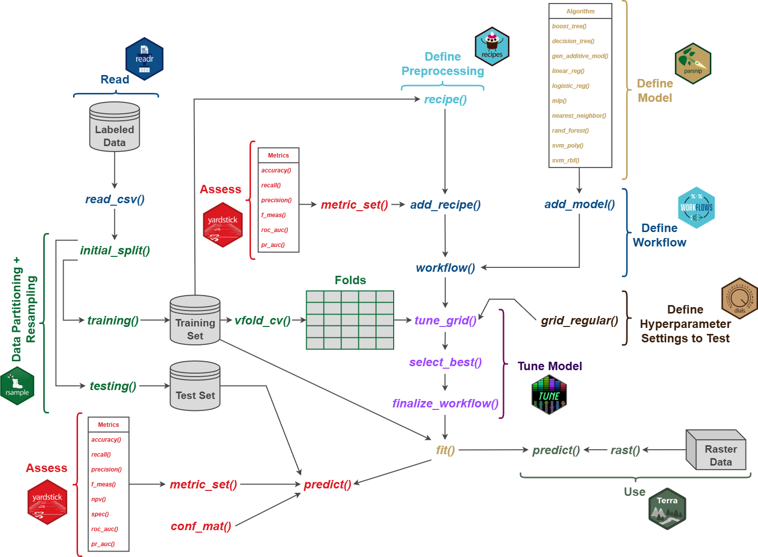
Expanding on the last chapter where we introduced tidymodels, this chapter explores two additional workflows. The first workflow integrates hyperparameter tuning using the rsample, tune, and dials packages. The process is simplified using the workflows package. The fourth and final workflow demonstrates the use of the workflowsets package for comparing different algorithm and preprocessing combinations. Before exploring these new workflows, we provide a brief introduction to hyperparameter tuning.
Below, we load all the required packages to execute the code in this chapter. Since this chapter uses the same data as Chapter 8, we only provided one copy of the data. So, we set our folder path to the Chapter 8 data folder.
fldPth <- "gslrData/chpt8/data/"9.3 Hyperparameter Tuning
One key component of the ML pipeline that we have not yet integrated is hyperparameter tuning. Hyperparameters are algorithm settings that are not learned during the training process. Examples include the number of trees in a decision tree (DT) ensemble model, the number of hidden layers in an artificial neural network (ANN), or the number of neighbors considered for k-nearest neighbors (kNN). In contrast, parameters are actually learned or updated during the training process. Examples include the splitting rules at each decision node in a DT and the weights and biases associated with a neuron in an ANN.
Since hyperparameters are not learned during the training process but often impact model performance, it is generally necessary to test different hyperparameter settings or hyperparameter settings combinations. This is the purpose of the tuning process.
9.3.1 Grid Search
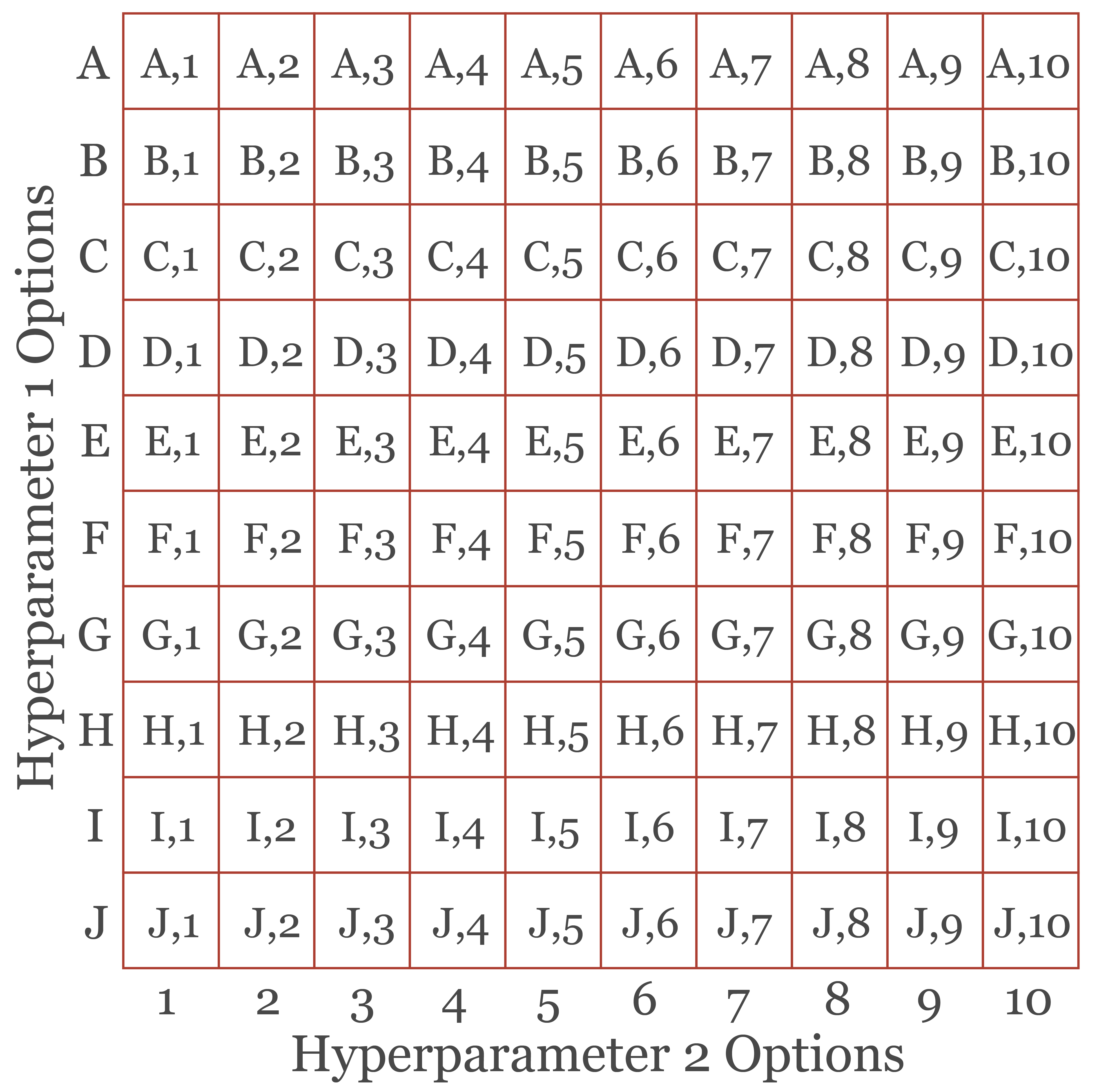
First, the user must determine (1) what hyperparameters need to be tuned for a specific algorithm and (2) which values or settings to test. All possible combinations of hyperparameters tested become the search space that must be assessed. Figure 9.1 conceptualizes a tuning grid with two hyperparameters. For Hyperparameter 1, values A through J are tested while values 1 through 10 are tested for Hyperparameter 2. The full set of combinations are specified by the grid visualized in the figure. Testing these combinations requires training and assessing a large number of models. Note that there are other means to select combinations to test other than every possible combination. However, we will focus on a full grid search here.
In tidymodels, the tune package is used to implement hyperparameter tuning while the dials package is used to manage hyperparameter settings.
9.3.2 Data Sampling
When testing hyperparameter setting combinations, assessing performance using the training set doesn’t make sense, as this would tend to select hyperparameter settings that result in overfitting to the training data. However, the test data should be reserved to assess the final model. There are several methods available to partition data for hyperparameter tuning.
Hold out: Instead of dividing the data into two partitions, three partitions are generated: training, validation, and test. The training set is used to train the model while the validation set is used to assess the model during hyperparameter tuning. The test set is withheld to assess the final model. A key drawback of this method is that it reduces the number of samples available to train the model.
-
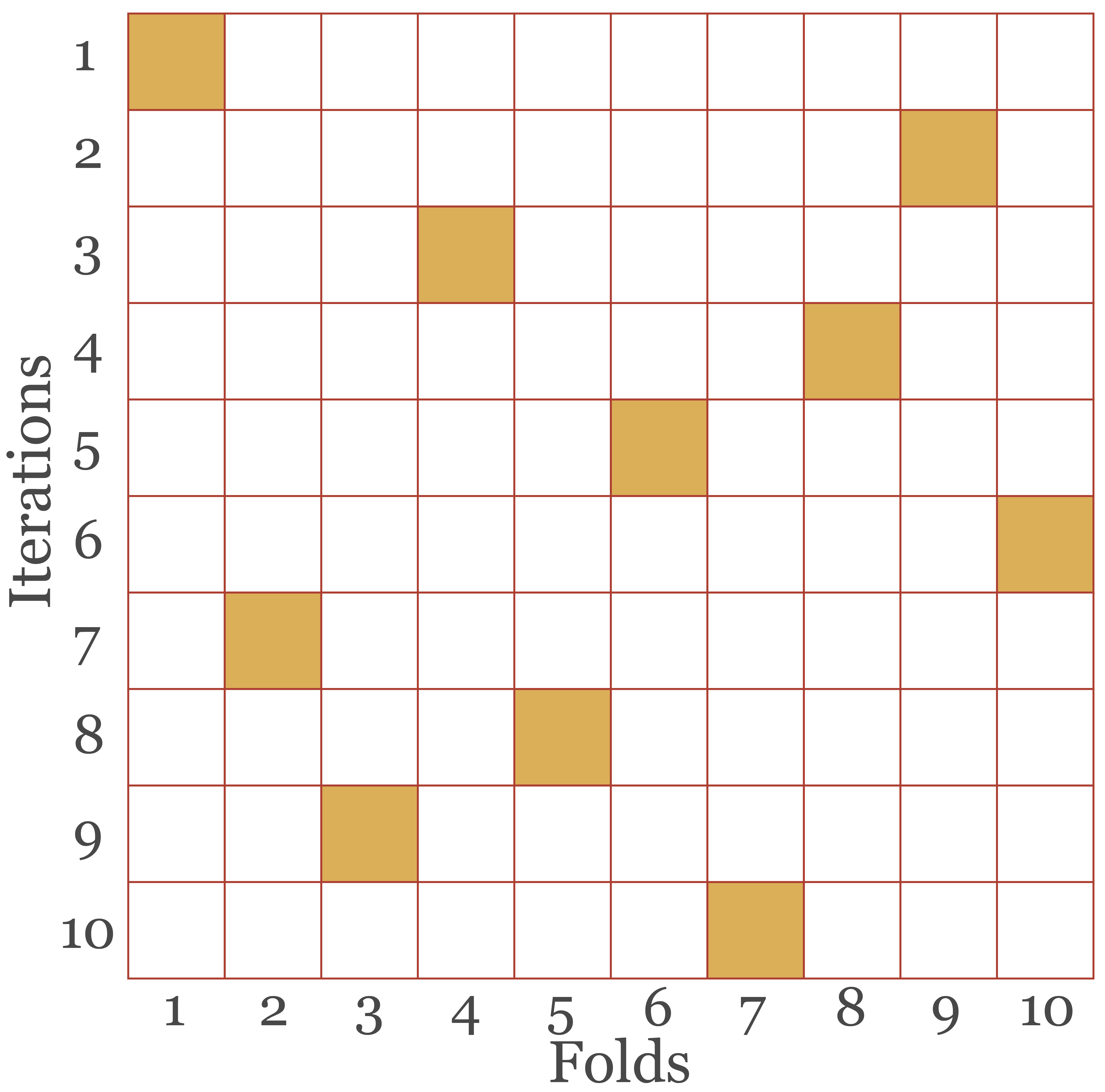
v-fold cross-validation (or k-fold cross validation): The training set is partitioned into non-overlapping folds where v is the number of folds. For each hyperparameter settings combination, the model is trained v times, each time training the model on all folds but one and using the withheld fold for model validation. The model is then trained using the selected optimal set of hyperparameter settings on the entire training set then assessed using the separate test set. This process can also make use of repeats, termed v-fold cross-validation with repeats, where new folds are generated for each repeat. Figure 9.2 conceptualizes 10-fold cross-validation where each square represents a fold. The data are partitioned into 10 non-overlapping folds (the columns of the grid). The model is then trained 10 times, which defines the rows of the table, each time withholding one fold for validation, differentiated for each iteration by the shaded square. The results are then averaged across all folds for each hyperparameter setting combination.
tidymodels uses the term v-fold cross-validation. However, this is more commonly referred to as k-fold cross-validation.
- Leave-one-out cross-validation: The model is trained n times, where n is the number of training samples. For each training iteration, n-1 samples are used to train the model and the remaining sample is withheld for validation. Assessment metrics are generated based on the aggregated results for the withheld samples. One drawback of this method is that it is computational intensive since a large number of models must be trained for each hyperparameter settings combination.
- Monte-Carlo cross-validation: This method uses random sampling without replacement to select a proportion of the training samples to train the model with the remainder used for validation. The user defines the number of repeats to use. In contrast to the folds used in v-fold cross validation, the training and validation partitions are not distinct between each Monte-Carlo replicate.
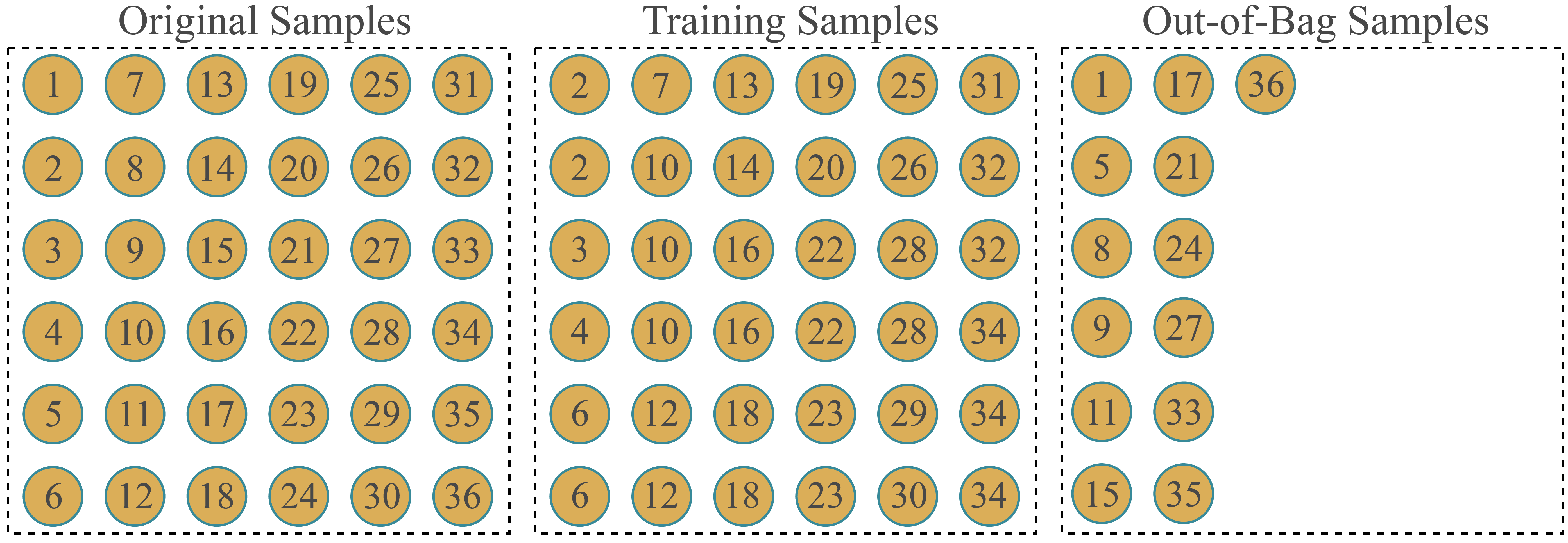
- Bootstrap resampling: This method makes use of random sampling with replacement to generate a training set equal in size to the full training set but with some repeating samples. The remaining samples are withheld for validation. Similar to Monte-Carlo cross-validation, the user defines the number of desired replicates. As conceptualized in Figure 9.3, the training set has the same size as the original training set due to repeat sampling of some observations. The number of withheld samples, termed out-of-bag (OOB) samples, that serve as the validation set will vary between replicates.
rsample provides functions to implement a variety of resampling methods including the following. Uppercase text indicates user inputs.
v-fold cross-validation =
vfold_cv(data = FULL TRAINING SET, v = NUMBER OF FOLDS, REPEATS = NUMBER OF REPEATS, strata = STATIFICATION VARIABLE FOR STRATIFIED RANDOM SAMPLING)Monte Carlo cross-validation =
mc_cv(data = FULL TRAINING SET, prop = PROPORTION TO INCLUDE IN TRAINING SET PER ITERATION, times = NUMBER OF REPLICATES, strata = STATIFICATION VARIABLE FOR STRATIFIED RANDOM SAMPLING)leave-one-out cross-validation =
loo_cv(data = FULL TRAINING SET)bootstrap sampling =
bootstraps(data = FULL TRAINING SET, times = NUMBER OF REPLICATES, strata = STATIFICATION VARIABLE FOR STRATIFIED RANDOM SAMPLING)
The code block below shows how to first split the full dataset into training and test partitions and then define folds, in this case 10-folds, for hyperparameter tuning using v-fold cross-validation.
monD <- read_csv(str_glue("{fldPth}monWFTable.csv")) |>
  mutate_if(is.character, as.factor) |>
  select(-OID_,
         -origComments,
         -CreationDate,
         -Creator,
         -EditDate,
         -Editor) |>
  drop_na()

set.seed(42)
monDStrat <- monD |>
  group_by(lcClass) |>
  sample_n(880,
           replace=FALSE) |>
  ungroup()

set.seed(42)
dataSplit <- monDStrat |>
  initial_split(prop=.7,
                strata=lcClass)

trainD <- training(dataSplit)

testD <- testing(dataSplit)

set.seed(42)
folds <- vfold_cv(trainD,
                  v = 10,
                  strata = lcClass)
It should also be mentioned that there are other means to define folds. For example, spatial proximity can be considered when defining folds in order to minimize spatial autocorrelation between folds. If you are interested in such methods, we recommend exploring the spatialsample package.
9.4 Workflow 3
We now explore the workflow conceptualized in Figure 9.4. The key difference between this and the workflows explored in the prior chapter is that we will now include hyperparameter tuning. In order to simplify this, we will make use of the workflows package. Note that it is not necessary to use workflows to implement hyperparameter tuning; however, we find that this simplifies the process, especially if you are also implementing preprocessing.
9.4.1 Data Partitioning
In the following code block we are (1) reading in the data; (2) augmenting the data by converting all character columns to factors, dropping unneeded columns, and removing rows with missing data; (3) extracting a stratified random sample to create a balanced dataset; and (4) partitioning the data into training and test sets using a 70/30 split, respectively. We are not implementing any preprocessing yet since we will now do this as part of the workflow.
monD <- read_csv(str_glue("{fldPth}/monWFTable.csv")) |>
  mutate_if(is.character, as.factor) |>
  select(-OID_,
         -origComments,
         -CreationDate,
         -Creator,
         -EditDate,
         -Editor) |>
  drop_na()

set.seed(42)
monDStrat <- monD |>
  group_by(lcClass) |>
  sample_n(880,
           replace=FALSE) |>
  ungroup()

set.seed(42)
dataSplit <- monDStrat |>
  initial_split(prop=.7,
                strata=lcClass)

trainD <- training(dataSplit)

testD <- testing(dataSplit)
9.4.2 Define Workflow
We now build a workflow that can be used to preprocess the data, tune hyperparameters, and train the model. We specifically work with the RF algorithm. The first step is to define a preprocessing pipeline using recipes. This involves defining the model (the land cover class, as represented by the “lcClass” column, will be predicted using all other variables in the table) and indicating to re-scale all numeric predictor variables. Note that this is not necessary for RF since it is not sensitive to data scale. We are simply including this here as an example.
In Workflow 2 from the last chapter, the next step was to use prep() and bake() to preprocess the training and test sets. These processes will now be completed inside of the workflow.
myRecipe <- recipe(lcClass ~ ., data = trainD) |>
  step_range(all_numeric_predictors())
We next define the RF model using parsnips and the "ranger" engine and make sure it is in "classification" mode. We set the number of trees in the model to 500, which means that this hyperparameter will not be tuned. Generally, RF does not overfit as more trees are added, so it is not generally important to tune this hyperparameter. Instead of either setting or using the default value for the number of random variables to select from at each decision node (mtry) and minimum number of data points in a node that are required for the node to be split further (min_n) hyperparameters, we use the tune() function to indicate that these hyperparameters should be tuned as part of the workflow.
rfSpec <- rand_forest(mtry=tune(),
                      min_n=tune(),
                      trees=500) |>
  set_engine("ranger") |>
  set_mode("classification")
We are now ready to define the workflow by adding the model and the preprocessing recipe. This results in a workflow object.
myWorkflow <- workflow() |>
  add_model(rfSpec) |>
  add_recipe(myRecipe)
9.4.3 Hyperparameter Tuning
Before using the workflow to tune hyperparameters, there are a few more steps required. First, we define a tuning grid of mtry and min_n value combinations to test. Here, we are testing 5 mtry values between 2 and 23. Note that the maximum value is the total number of predictor variables, which is 23 in this case. For min_n, we test three values between 2 and 10. This results in a total of 15 combinations that need to be tested. It would be preferable to test more combinations; however, this will take longer to execute, so we are simplifying the tuning process for the sake of time.
We next define folds from the training set. We use 10-fold cross-validation without repeats and stratify on the land cover classes in order to maintain the class proportions between the folds. Given that this is a balanced dataset, this is not actually necessary.
set.seed(42)
folds <- vfold_cv(trainD,
                  v = 10,
                  strata = lcClass)
Lastly, we need to define metrics that will be used to assess model performance with different hyperparameter combinations. Specifically, we will calculate overall accuracy and macro-averaged F1-score, precision, and recall. This is accomplished using the metric_set() function from yardstick.
myMetrics <- metric_set(accuracy,
                        f_meas,
                        precision,
                        recall)
We are now ready to tune the model. For this experiment, this requires testing a total of 15 hyperparameter settings combinations using 10 iterations where one fold is withheld and the other 9 folds are used to train the model. Thus, we need to train 150 models. To speed up the process, we implement parallel computing using the doParallel package, which requires using a machine with multiple CPU cores. The tuning process is implemented using the tune_grid() function from the tune package, which requires providing a workflow object, data resamples or folds, a grid of hyperparameter setting combinations to test, and assessment metrics, all of which were defined above.
Note that this will take some time to execute if you choose to execute the code.
doParallel::registerDoParallel()

set.seed(123)
rf_tuning_results <- tune_grid(
  myWorkflow,
  resamples = folds,
  grid = rf_grid,
  metrics = myMetrics
)
9.4.4 Finalize Workflow
Once the tuning process is completed, we can select the best hyperparameter combination using the select_best() function from the tune package.
best_rf_params <- rf_tuning_results |>
  select_best(metric = "f_meas")
Now that we have tuned the model, it can be finalized using the finalize_workflow() function from tune. If we were tuning a model outside of a workflow, we would use the finalize_model() function. Once the workflow is finalized, the model can be trained with fit() using the entire training set and the hyperparameter settings selected by the tuning process.
myWorkflowFinal <- myWorkflow |>
  finalize_workflow(best_rf_params)
rfModel <- myWorkflowFinal |>
fit(data = trainD)9.4.5 Model Assessment
We have now implemented the complete process required to train the model including data preprocessing, hyperparameter tuning, and training. We can now validate the final model using the withheld test data. This involves first obtaining predictions for the test data using predict() then using the reference labels and predictions to calculate assessment metrics with yardstick. We can also obtain the complete confusion matrix using conf_mat().
testPred |>
  myMetrics(truth = lcClass,
            estimate = .pred_class) |>
gt()| .metric | .estimator | .estimate |
|---|---|---|
| accuracy | multiclass | 0.9375000 |
| f_meas | macro | 0.9372432 |
| precision | macro | 0.9388865 |
| recall | macro | 0.9375000 |
testPred |>
  conf_mat(truth = lcClass,
           estimate = .pred_class)
Truth
Prediction barren conForest decForest developed grass water
barren 248 0 0 25 6 6
conForest 0 253 2 3 1 1
decForest 1 5 262 3 1 3
developed 9 1 0 219 3 4
grass 6 5 0 13 253 0
water 0 0 0 1 0 2509.5 Workflow 4
In this final workflow, we compare workflows that use different preprocessing and algorithm combinations. We implement all of the components from the prior workflows including data partitioning, preprocessing, hyperparameter tuning, and model validation. In order to define different workflow combinations, we make use of the workflowsets package.
9.5.1 Preparation
The code block below is the same as the prior example and accomplishes the following:
- Read in the data
- Augment the data table by converting all character columns to factors, dropping unneeded columns, and removing rows with missing data
- Extract a stratified random sample to create a balance dataset
- Partition the data into training and test sets using a 70/30 split, respectively
monD <- read_csv(str_glue("{fldPth}/monWFTable.csv")) |>
  mutate_if(is.character,
            as.factor) |>
  select(-OID_,
         -origComments,
         -CreationDate,
         -Creator,
         -EditDate,
         -Editor) |>
  drop_na()

set.seed(42)
monDStrat <- monD |>
  group_by(lcClass) |>
  sample_n(100,
           replace=FALSE) |>
  ungroup()

set.seed(42)
dataSplit <- monDStrat |>
  initial_split(prop=.7,
                strata=lcClass)

trainD <- training(dataSplit)

testD <- testing(dataSplit)
We next defined training set folds using 10-fold cross-validation for use during hyperparameter tuning.
set.seed(123)
folds <- vfold_cv(trainD,
                  v = 10,
                  repeats=1,
                  strata = lcClass)
9.5.2 Define Workflowset
We will experiment with two different preprocessing routines. As we did in the last two workflows, we will re-scale all the numeric predictor variables using step_range(). As a second preprocessing routine, we will apply both normalization and principal component analysis (PCA) for feature reduction. We specifically extract the first ten principal components.
myRecipeNorm <- recipe(lcClass ~ .,
                       data=trainD) |>
  step_range(all_numeric_predictors())

myRecipePCA <- recipe(lcClass ~ .,
                      data = trainD) |>
  step_normalize(all_numeric_predictors()) |>
  step_pca(all_numeric_predictors(),
           trained=FALSE,
           num_comp = 10)
We will compare four different models: RF, SVM with an RBF kernel, kNN, and a DT. All the models are specified using parsnips and placed in classification mode. Any hyperparameters that need to be tuned are specified using tune().
rfSpec <- rand_forest(mtry=tune(),
                      min_n=tune(),
                      trees=500) |>
  set_engine("ranger") |>
  set_mode("classification")

svmSpec  <-
  svm_rbf(cost = tune(),
          rbf_sigma = tune()) |>
  set_engine("kernlab") |>
  set_mode("classification")

knnSpec <-
  nearest_neighbor(neighbors = tune(),
                   dist_power = tune(),
                   weight_func = tune()) |>
  set_engine("kknn") |>
  set_mode("classification")

dtSpec <-
  decision_tree(cost_complexity = tune(),
                min_n = tune()) |>
  set_engine("rpart") |>
  set_mode("classification")
We have now specified four algorithms to compare and two preprocessing routines, or a total of 8 combinations. Within the workflow_set() function, preprocessing routines to test are provided as a list object for the preproc parameter while a list of model objects are provided as the argument for the models parameter.
9.5.3 Hyperparameter Tuning
In order to tune the hyperparameters, we first set tuning controls using the control_grid() function. We will parallel over "everything" in order to speed up the process. When verbose is set to TRUE, information will be printed during the tuning process.
The tuning process is implemented using workflow_map(), which requires specifying the training set folds, the tuning controls, and the metrics to use in the evaluation. We set a random seed for reproducibility. Setting the grid argument to 10 indicates that ten values for each hyperparameter will be tested. Another option is to specify your own settings or values to test. However, we generally find this setup to be adequate.
If you choose to execute this code, it will take some time. So, please be patient.
myMetrics <- metric_set(accuracy,
                        f_meas)

grid_ctrl <-
  control_grid(
    verbose=FALSE,
    save_pred = TRUE,
    parallel_over = "everything",
    save_workflow = TRUE
  )

grid_results <-
  myWFS |>
  workflow_map(
    seed = 42,
    resamples = folds,
    grid = 10,
    control = grid_ctrl,
    metrics=myMetrics
  )
The autoplot() function can be applied to the tuning results to visualize the outcomes.
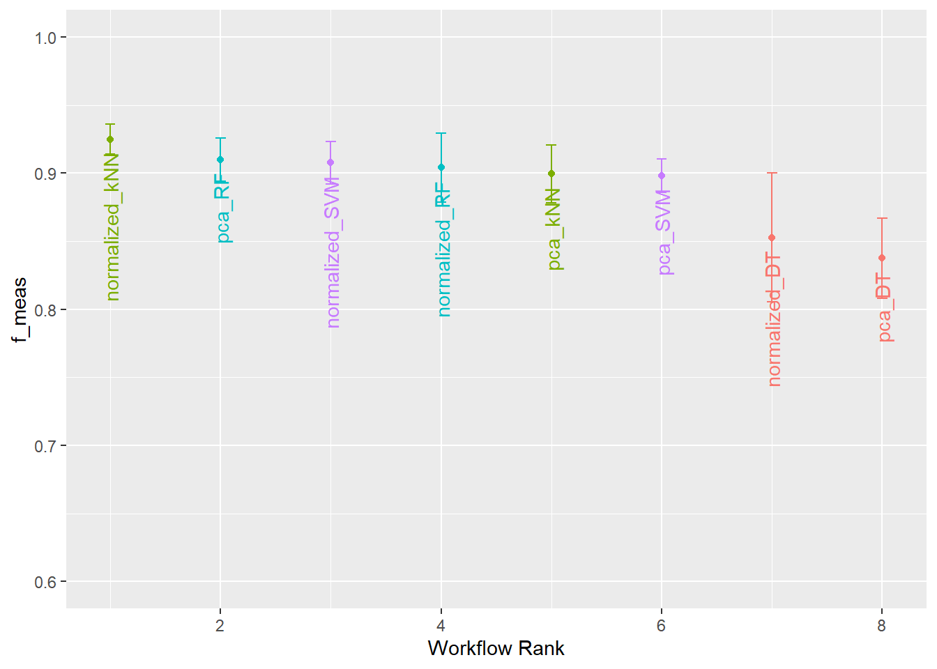
9.5.4 Fit Final Models
Once the models have been tuned, we can extract the desired model using extract_workflow_set_result(), select the best hyperparameters using select_best(), finalize the workflow with finalize_workflow(), and fit the model using the entire training set using fit(). This results in a final fitted model that can be used to make predictions. In the example, we are finalizing the RF model + re-scale preprocessing combination since it performed well.
rfResults <- grid_results |>
  extract_workflow_set_result("normalized_RF") |>
  select_best(metric="f_meas")

rfModel <-
  grid_results |>
  extract_workflow(id="normalized_RF") |>
  finalize_workflow(rfResults) |>
  fit(data = trainD)
9.5.5 Assess Model
9.5.5.1 Assess with yardstick
Model assessment of the final model can be performed using the same process as used in the prior two workflows. First, it is necessary to predict the test samples using predict() then use the reference labels and predictions to calculate assessment metrics using yardstick.
testPred |>
  myMetrics(truth = lcClass,
            estimate = .pred_class) |>
gt()| .metric | .estimator | .estimate |
|---|---|---|
| accuracy | multiclass | 0.8277778 |
| f_meas | macro | 0.8250019 |
testPred |>
  conf_mat(truth = lcClass,
           estimate = .pred_class)
Truth
Prediction barren conForest decForest developed grass water
barren 26 0 0 7 4 1
conForest 0 29 0 2 0 2
decForest 0 1 29 0 2 0
developed 4 0 1 17 3 0
grass 0 0 0 4 21 0
water 0 0 0 0 0 279.5.5.2 Assess with micer
If you need to conduct additional comparisons, it is possible to extract multiple models from the workflow set. Below, we are extracting out two models, kNN + re-scale and RF + re-scale, selecting the best hyperparameters, finalizing their associated workflows, and fitting the model using the entire training set. We then use the trained models to make predictions for the withheld test set and calculate assessment metrics.
rfResults <- grid_results |>
  extract_workflow_set_result("normalized_RF") |>
  select_best(metric="f_meas")

rfModel <-
  grid_results |>
  extract_workflow(id="normalized_RF") |>
  finalize_workflow(rfResults) |>
  fit(data = trainD)

kNNResults <- grid_results |>
  extract_workflow_set_result("normalized_kNN") |>
  select_best(metric="f_meas")

kNNModel <-
  grid_results |>
  extract_workflow(id="normalized_kNN") |>
  finalize_workflow(kNNResults) |>
  fit(data = trainD)

rfPred <- rfModel |>
  predict(testD) |>
  bind_cols(testD)

kNNPred <- kNNModel |>
  predict(testD) |>
  bind_cols(testD)
We can also statistically compare the models based on map image classification efficacy (MICE) via the miceCompare() function from micer.
miceCompare(ref=rfPred$lcClass,
            result1=rfPred$.pred_class,
            result2=kNNPred$.pred_class,
            reps=2000,
            frac=.4) |>
  print()
    Paired t-test

data:  resultsDF$mice1 and resultsDF$mice2
t = -29.318, df = 1999, p-value < 2.2e-16
alternative hypothesis: true mean difference is not equal to 0
95 percent confidence interval:
 -0.03464414 -0.03029989
sample estimates:
mean difference
    -0.03247202
9.5.6 Workflow Sets for Experimentation
One of the great values of workflow sets is the ability to perform well controlled experiments using consistent and clean code. Below, we describe how to define a few example workflow sets to answer some specific research questions.
9.5.6.1 Question 1
The following workflow set could be used to compare model performance when using all spectral variables, just the leaf-on bands, and just the leaf-off bands. This is accomplished by defining three separate recipes. The step_select() function is used to filter out a subset of predictor variables. In this test, we are only using the RF algorithm.
recipeSpec <- recipe(lcClass ~ ., data=trainD) |>
  step_select(-elev, -slp, -tpi)
recipeON <- recipe(lcClass ~ ., data=trainD) |>
  step_select(contains("_may"))
recipeOFF <- recipe(lcClass ~ ., data=trainD) |>
  step_select(contains("_apr"))

rfSpec <- rand_forest(mtry=tune(),
                      min_n=tune(),
                      trees=500) |>
  set_engine("ranger") |>
  set_mode("classification")

myWFS <-
  workflow_set(
    preproc = list(specVars=recipeSpec,
                   leafOn = recipeON,
                   leafOff = recipeOFF),
    models = list(RF = rfSpec)
  )
9.5.6.2 Question 2
This workflow could be used to explore how a model using all variables compares to a model that only uses the spectral variables. Comparisons between these two different feature spaces are made for four algorithms.
recipeAll <- recipe(lcClass ~ ., data=trainD)
recipeSpec <- recipe(lcClass ~ ., data=trainD) |>
    step_select(-elev, -slp, -tpi)

rfSpec <- rand_forest(mtry=tune(),
                      min_n=tune(),
                      trees=500) |>
  set_engine("ranger") |>
  set_mode("classification")

svmSpec  <-
  svm_rbf(cost = tune(),
          rbf_sigma = tune()) |>
  set_engine("kernlab") |>
  set_mode("classification")

knnSpec <-
  nearest_neighbor(neighbors = tune(),
                   dist_power = tune(),
                   weight_func = tune()) |>
  set_engine("kknn") |>
  set_mode("classification")

dtSpec <-
  decision_tree(cost_complexity = tune(),
                min_n = tune()) |>
  set_engine("rpart") |>
  set_mode("classification")

myWFS <-
  workflow_set(
    preproc = list(allVars = recipeAll,
                   specVars = recipeSpec),
    models = list(RF = rfSpec,
                  SVM = svmSpec,
                  kNN = knnSpec,
                  DT = dtSpec)
  )
9.5.6.3 Question 3
In this workflow, we are using a single preprocessing recipe but varying the model. Specifically, we are investigating the performance of the kNN model when using different numbers of neighbors: 7, 11, and 21. A similar comparison could be done using hyperparameter tuning.
recipeAll <- recipe(lcClass ~ ., data=trainD)

knn7 <-
  nearest_neighbor(neighbors = 7) |>
  set_engine("kknn") |>
  set_mode("classification")

knn11 <-
  nearest_neighbor(neighbors = 11) |>
  set_engine("kknn") |>
  set_mode("classification")

knn21 <-
  nearest_neighbor(neighbors = 21) |>
  set_engine("kknn") |>
  set_mode("classification")

myWFS <-
  workflow_set(
    preproc = list(allVars = recipeAll),
    models = list(knn7 = knn7,
                  knn11 = knn11,
                  knn21 = knn21)
  )
9.5.6.4 Question 4
In this last example, we compare the impact of using three different feature reduction methods: principal component analysis (PCA), kernel principal component analysis (kPCA), and independent component analysis (ICA). A total of 11 components are used for each method for consistency, and they are calculated from only the spectral variables. The three different feature reduction methods are evaluated for both the RF and SVM algorithms.
recipePCA <- recipe(lcClass ~ ., data=trainD) |>
  step_select(-elev, -slp, -tpi) |>
  step_pca(num_comp=11)

recipeKPCA <- recipe(lcClass ~ ., data=trainD) |>
  step_select(-elev, -slp, -tpi) |>
  step_kpca(num_comp=11)

recipeICA <- recipe(lcClass ~ ., data=trainD) |>
  step_select(-elev, -slp, -tpi) |>
  step_ica(num_comp=11)

rfSpec <- rand_forest(mtry=tune(),
                      min_n=tune(),
                      trees=500) |>
  set_engine("ranger") |>
  set_mode("classification")

svmSpec  <-
  svm_rbf(cost = tune(),
          rbf_sigma = tune()) |>
  set_engine("kernlab") |>
  set_mode("classification")

myWFS <-
  workflow_set(
    preproc = list(pca = recipePCA,
                   kpca = recipeKPCA,
                   ica = recipeICA),
    models = list(RF = rfSpec,
                  SVM = svmSpec)
  )
9.6 Closing Remarks
We hope you found the last two chapters associated with the tidymodels metapackage useful. If you are interested in learning more about tidymodels, we recommend Tidy Modeling with R by Kuhn and Silge. The tidymodels documentation is also excellent.
9.7 Questions
- Explain why withholding validation data is necessary when performing hyperparameter tuning.
- Explain the difference between v-fold cross-validation and v-fold cross validation with repeats.
- Explain the difference between Monte Carlo cross-validation and bootstrap resampling.
- When performing hyperparameter tuning, explain the purpose of the rsample, tune, and dials packages.
- For a workflow, what is the purpose of the
select_best()function? - For a workflow, what is the purpose of the
finalize_workflow()function? - What is the purpose of
add_model()andadd_recipe()for a workflow object? - Explain the difference between a workflow and a workflowset.
9.8 Exercises
This exercise expands upon the Chapter 8 exercise. Before beginning this exercise, perform the same preprocessing steps as those undertaken in Chapter 8. Expanding upon the Chapter 8 activity, you will now use workflowsets to further preprocess, tune, and compare models.
Models to Compare
Compare the following models:
- Random forest
- Support vector machine with an RBF kernel
- Support vector machine with a polynomial kernel
- k-nearest neighbors
Feature Spaces
Compare models using all 15 predictor variables with models using only the spectral bands: “Blue”, “Green”, “Red”, and “NIR”.
Tuning Requirements
Tune the following hyperparameters for the algorithms/feature space combinations. For random forest, use 500 trees. You can use default arguments for all other parameters. Test 10 values for each hyperparameter using grid=10. Calculate overall accuracy and class-aggregated, macro-averaged F1-score, precision, and recall. For each algorithm, select the hyperparameters that provide the highest F1-score.
- Random forest
mtry
- Support vector machine (RBF)
costrbf_sigma
- Support vector machine (Polynomial)
costdegree
-
k-nearest neighbor
neighbors
Assess Models
For all 8 model and feature space combinations, finalize the models by fitting them using the entire training set with the selected hyperparameters. Use the finalized models to make predictions to the test data. Use the predictions and test reference labels to calculate overall accuracy and macro-average, class-aggregated F1-score, precision, and recall. Also generate confusion matrices for all 8 models.
Produce a short write up that summarizes your comparisons. What had a larger impact, the algorithm used or the feature space? How might you further improve the model?