12 Convolutional Neural Network (Scene Classification)
12.1 Topics Covered
- Prepare data for use in a torch/luz workflow
- Build a dataset subclass appropriate for training a convolutional neural network (CNN)
- Build a CNN by subclass
nn_module() - Understand the use and parameterization of the following layer types: 2D convolutional layers (
nn_conv2d()), batch normalization (nn_batchnorm1d()andnn_batchnorm2d()), 2D max pooling (nn_maxpool2d()), linear or fully connected (nn_linear()), and rectified linear unit (ReLU) activation function (nn_relu()) - Train a CNN using luz
- Define loss metrics and optimizers
- Assess CNN results using withheld data and assessment metrics
- Use a pre-defined CNN architecture (ResNet-32) provided by the torchvision package
- Load pre-trained model parameters and freeze model components
- Augment a pre-defined model architecture
- Generally understand the shape and dimensionality of input, output, and intermediate tensors as data are processed by a CNN
12.2 Introduction
This chapter explores the same problem demonstrated in the last chapter: the land cover classification of 640-by-640 m Sentinel-2 Multispectral Instrument (MSI) image chips from the EuroSat dataset. However, we now use a convolutional neural network (CNN) architecture as opposed to a fully connected architecture. This allows us to treat the image data as images as opposed to collapsing them into a tabular form. Reminder that the EuroSat dataset is available on GitHub and Kaggle. This paper introduced the data. These data have not been provided as part of this text. We recommend downloading them from Kaggle.
12.3 Data Preparation
12.3.1 Loading and Preprocessing
We begin with some data preparation. The originators of the dataset have already divided the samples into training, validation, and test sets, which are listed out in provided CSV files. Those files are read in using readr. Printing the number of rows in each tibble, we can see that there are 19,317 training, 5,519 validation, and 2,759 test samples. Each table provides the file name (“Filename”), class numeric label (“Label”), and class name (“ClassName”). As already described in the last chapter, there are a total of ten land cover classes differentiated.
| Filename | Label | ClassName |
|---|---|---|
| PermanentCrop/PermanentCrop_2401.tif | 6 | PermanentCrop |
| PermanentCrop/PermanentCrop_1006.tif | 6 | PermanentCrop |
| HerbaceousVegetation/HerbaceousVegetation_1025.tif | 2 | HerbaceousVegetation |
| SeaLake/SeaLake_1439.tif | 9 | SeaLake |
| River/River_1052.tif | 8 | River |
| Forest/Forest_2361.tif | 1 | Forest |
12.3.2 Define Dataset Subclass
The dataset subclass defined in the last chapter will not work here since we are now working with the image chips as opposed to band means. For our new subclass, the .getitem() method must return a tensor representing a single image with the shape [# of bands, # of rows, # of columns]. Since there is still only a single label assigned to each chip, the label tensor will be the same as that used in the last chapter.
The code block below defines the new subclass eurosatDataSet(). The user can define (1) the name of the data frame/tibble that lists the image names and associated labels, (2) the path to the data, (3) the indices for the bands that will be included as predictor variables, and (4) whether or not to perform data augmentations.
There are two version of the EuroSat dataset. We are using the EuroSATallBands version as opposed to the EuroSAT version, which only includes the red, green, and blue channels.
The .getitem() method generates a single sample consisting of a tensor representing the image data and a tensor representing the class label. This is accomplished as follows:
- The image name is extracted from data frame/tibble
- The numeric label is extracted from the data frame/tibble and converted to a torch tensor with a long integer (
torch_int64()) data type; 1 is added to the label numeric code since R starts indexing at 1 as opposed to 0; dimensions with a length of one are removed usingsqueeze() - The raster image is read using the
rast()function from terra; the desired bands are extracted; the raster image is converted to an R array; and the array is converted to a torch tensor with atorch_float32()data type - Since terra uses [rows, columns, channels] as opposed to [channels, rows, columns], as expected by torch,
permute()is used to change the dimension order - The image data are rescaled by dividing by 10,000
- If augmentations are desired, torchvision is used to apply random horizontal and vertical flips.
- The two tensors are returned inside of a list object
The .length() method returns the number of available samples, in this case the number of rows in the table.
eurosatDataSet <- torch::dataset(

  name = "eurosatDataSet",

  initialize = function(df,
                        pth,
                        bands,
                        doAugs=FALSE){
    self$df <- df
    self$pth <- pth
    self$bands <- bands
    self$doAugs <- doAugs
  },

  .getitem = function(i){

    imgName <- unlist(self$df[i, "Filename"], use.names=FALSE)

    label <- unlist(self$df[i, "Label"], use.names=FALSE) |>
      torch_tensor(dtype=torch_int64()) |>
      torch_add(1)
    label <- label$squeeze()
    label <- label |> torch_tensor(dtype=torch_int64())

    img <- rast(paste0(self$pth, imgName)) |>
      terra::subset(self$bands) |>
      as.array() |>
      torch_tensor(dtype=torch_float32())

    img <- img$permute(c(3,2,1))

    img <- img/10000

    if(self$doAugs == TRUE){
      img <- torchvision::transform_random_horizontal_flip(img, p=0.5)

      img <- torchvision::transform_random_vertical_flip(img, p=0.5)
    }

    return(list(preds = img, label = label))
  },

  .length = function(){

    return(nrow(self$df))

  }
)
12.3.3 Define Datasets and Dataloaders
We now instantiate the three datasets. Instead of using all 13 bands, we subset out 10 bands: blue, green, red, red edge 1, red edge 2, red edge 3, near infrared (NIR), narrow NIR, shortwave infrared 1 (SWIR1), and SWIR2. Since augmentations are used in an attempt to minimize overfitting, they are only applied for the training set.
Once the datasets are defined, dataloaders are generated with a mini-batch size of 32. If you execute the training loop, you may need to change this mini-batch size depending on your hardware specifications. The training set is shuffled to combat overfitting. We drop the last mini-batch for the training and validation dataloaders since they may have a different length than the other mini-batches. The test dataloader uses all samples so that all predictions can be compared to the correct labels to generate assessment metrics.
trainDL <- torch::dataloader(trainDS,
                             batch_size=32,
                             shuffle=TRUE,
                             drop_last = TRUE)

valDL <- torch::dataloader(valDS,
                           batch_size=32,
                           shuffle=FALSE,
                           drop_last = TRUE)

testDL <- torch::dataloader(testDS,
                            batch_size=32,
                            shuffle=FALSE,
                            drop_last = FALSE)
Before moving on, we next explore a single mini-batch to make sure there are no issues. The shape of the image tensor is [32, 10, 64, 64]: each mini-batch consists of 32 samples, each with 10 channels and 64-by-64 pixels. The label tensor has a shape of [32] since only a single numeric label is required for each sample. The image tensor has a float data type while the labels have a long integer data type. Lastly, we print the band means, which confirms that the digital numbers have been rescaled. In short, everything looks good.
batch1 <- trainDL$.iter()$.next()

batch1$preds$shape
[1] 32 10 64 64batch1$label$shape[1] 32batch1$preds$dtypetorch_Floatbatch1$label$dtypetorch_Longtorch_mean(batch1$preds, dim=c(1,3,4))torch_tensor
0.1107
0.1014
0.0894
0.1118
0.1882
0.2257
0.2177
0.0624
0.1042
0.2483
[ CPUFloatType{10} ]12.4 CNN From Scratch
12.4.1 Define Architecture
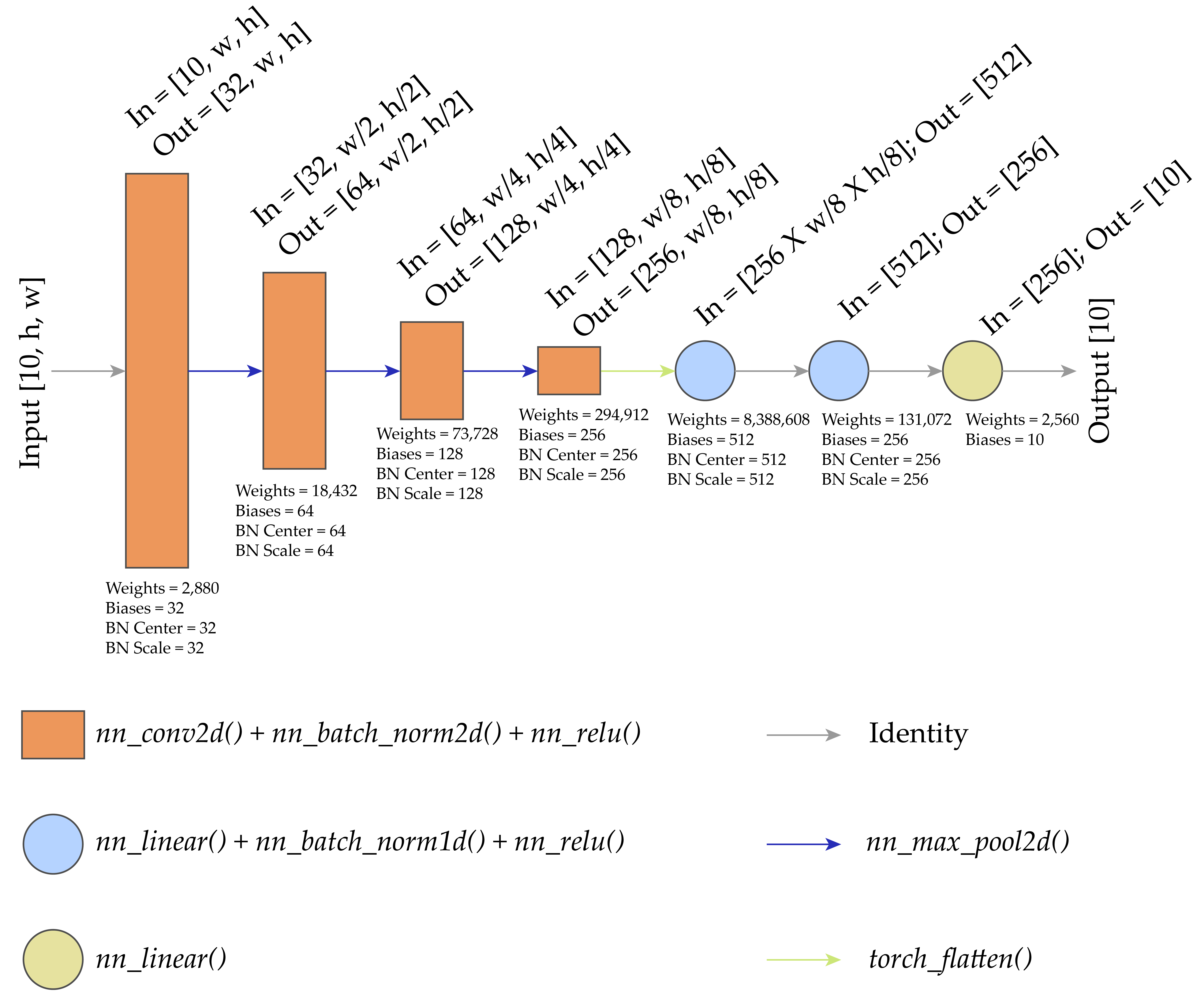
We now define the CNN architecture conceptualized in Figure 12.1. This architecture consists of the following:
- Four convolutional layers consisting of 2D convolution, 2D batch normalization, and a rectified linear unit (ReLU) activation
- 2D max pooling after the first 3 convolutional layers to decrease the size of the array in the spatial dimensions
- Flattening the result from the 4th convolutional layer to a 1D array prior to passing it to the fully connected component of the architecture
- Three fully connected layers with 512, 256, and 10 nodes/neurons, respectively
The number of weights in each 2D convolutional layer is equal to the kernel size (3x3) multiplied by the number of input and output feature maps. The number of bias terms is equal to the number of output feature maps for the convolutional layer. For the 2D batch normalization, both the number of scale and shift parameters is equal to the number of output feature maps. 2D max pooling, ReLU activation, and flattening do not have trainable parameters.
The number of inputs accepted by the first fully connected layer is equal to 8 x 8 x number of output feature maps from the final convolutional layer. This is because the array will have spatial dimensions of 8-by-8 cells after the final 2D max pooling is applied (64-by-64 –> 32-by-32 –> 16-by-16 –> 8-by-8). It is important to note that the size of the flattened array will be different if the original input size is different. In other words, this network would need to be modified to accept input data with a different count of rows and columns of pixels. If data are to be fed into the network that do not have a consistent size, resampling and/or cropping would need to be applied to standardize their sizes and/or aspect ratios.
The last fully connected layer has 10 nodes/neurons since we are differentiating 10 classes. Since no softmax activation is applied, raw logits are returned.
12.4.1.1 Subclass nn_module
The model architecture is defined by subclassing nn_module(). The user can defined (1) the number of input channels, (2) the number of feature maps produced by each convolutional layer, (3) the number of nodes/neurons in the first two fully connected layers, and (4) the number of output class, which also defines the number of nodes/neurons in the final fully connected layer. We have provided default arguments for all parameters.
nn_sequential() has been used to build the model in two pieces: the convolutional component and the fully connected component. 2D convolution is performed using nn_conv2d() with a kernel size of 3x3. The padding is set to 1 to maintain the size of the array in the spatial dimensions. For each convolutional layer, the number of input channels or feature maps and number of output feature maps must be defined. After all four convolution operations, 2D batch normalization and a ReLU activation are applied using nn_batch_norm2d() and nn_relu(). The convolutional component of the architecture is named cnnComp().
The fully connected component, named fcComp(), makes use of the following layer types: nn_linear(), nn_batchnorm1d(), and nn_relu(). nn_linear() requires the number of input values and number of nodes/neurons in the layer, which is equivalent to the number of values that are passed to the next layer in the architecture.
The input parameters and two components of the model are defined/initialized within the initialize() method while the forward() method defines how data will pass through the architecture. The data, x, first pass through the convolutional component. Next, they are flattened using torch_flatten() such that a single sample in a mini-batch becomes a 1D vector but each separate sample is maintained as a separate vector. Lastly, the data pass through the fully connected component of the architecture.
myCNN <- nn_module(
  "convnet",

  initialize = function(inChn=3,
                        nFMs=c(32, 64, 128, 256),
                        nNodes=c(512, 256),
                        nCls=3) {

    self$inChn = inChn
    self$nFMs = nFMs
    self$nNodes = nNodes
    self$nCls = nCls

    self$cnnComp <- nn_sequential(
      nn_conv2d(inChn, nFMs[1], kernel_size=3, padding=1),
      nn_batch_norm2d(nFMs[1]),
      nn_relu(),
      nn_max_pool2d(kernel_size=2),
      nn_conv2d(nFMs[1], nFMs[2], kernel_size=3, padding=1),
      nn_batch_norm2d(nFMs[2]),
      nn_relu(),
      nn_max_pool2d(kernel_size=2),
      nn_conv2d(nFMs[2], nFMs[3], kernel_size=3, padding=1),
      nn_batch_norm2d(nFMs[3]),
      nn_relu(),
      nn_max_pool2d(kernel_size=2),
      nn_conv2d(nFMs[3], nFMs[4], kernel_size=3, padding=1),
      nn_batch_norm2d(nFMs[4]),
      nn_relu()
    )

    self$fcComp <- nn_sequential(
      nn_linear(nFMs[4]*8*8, nNodes[1]),
      nn_batch_norm1d(nNodes[1]),
      nn_relu(),
      nn_linear(nNodes[1], nNodes[2]),
      nn_batch_norm1d(nNodes[2]),
      nn_relu(),
      nn_linear(nNodes[2], nCls),
    )

  },

  forward = function(x) {

    x <- self$cnnComp(x)
    x <- torch_flatten(x, start_dim = 2)
    x <- self$fcComp(x)
    return(x)

  }
)
12.4.1.2 Explore Model
Now that the architecture has been built, an instance of it can be instantiated. We have configured the instance to work with the EuroSat data. Specifically, it expects 10 input channels and returns 10 class logits. Next, we pass some random example data through the model with the correct shape ([32, 10, 64, 64]) and obtain the shape of the prediction, which is [32,10]: 10 logits, one for each class, is predicted for each sample in the mini-batch of 32 samples.
testT <- torch_rand(32, 10, 64, 64)
testTPred <- model(testT)

testTPred$shape
[1] 32 10Table 12.1 highlights the number of trainable parameters in each layer in the architecture for the EuroSat configuration. Interestingly, the first fully connected layer has the largest number of trainable parameters. This is because of the large number of inputs (8x8x256) for this layer following the flattening of the tensor arrays. We also confirm the total count of trainable parameters using a custom function. The architecture contains 8,915,946 trainable parameters, which include kernel weights and biases, batch normalization scale and shift, and fully connected layer weights and biases.
| Layer | Weights | Biases | BN Scale | BN Shift |
|---|---|---|---|---|
| Convolution 1 | 2,880 | 32 | 32 | 32 |
| 2D Max Pool 1 | 0 | 0 | 0 | 0 |
| Convolution 2 | 18,432 | 64 | 64 | 64 |
| 2D Max Pool 2 | 0 | 0 | 0 | 0 |
| Convolution 3 | 73,728 | 128 | 128 | 128 |
| 2D Max Pool 3 | 0 | 0 | 0 | 0 |
| Convolution 4 | 294,912 | 256 | 256 | 256 |
| Flatten | 0 | 0 | 0 | 0 |
| Fully Connected 1 | 8,388,608 | 512 | 512 | 512 |
| Fully Connected 2 | 131,072 | 256 | 256 | 256 |
| Fully Connected 3 | 2,560 | 10 | 0 | 0 |
| Total | 8,912,192 | 1,258 | 1,248 | 1,248 |
| Grand Total | 8,915,946 |
count_trainable_params <- function(model) {
  if (!inherits(model, "nn_module")) {
    stop("The input must be a torch nn_module.")
  }

  params <- model$parameters

  trainable_params <- lapply(params, function(param) {
    if (param$requires_grad) {
      as.numeric(prod(param$size()))
    } else {
      0
    }
  })

  total_trainable_params <- sum(unlist(trainable_params))

  return(total_trainable_params)
}count_trainable_params(model)[1] 891594612.4.2 Train Model with luz
Now that we have datasets and dataloaders defined for the EuroSat dataset and built an appropriate model architecture, we are ready to train the model. As we did in the last chapter, we will train the model using luz as opposed to building a custom training loop. Within setup() we indicate that we will use cross entropy (CE) loss via nn_cross_entropy_loss(), the AdamW optimizer, and monitor the overall accuracy using luz_metric_accuracy().
set_hparams() defines the same hyperparameters as used above for the CNN architecture. The model is fit using the trainDL dataloader and validated on the valDL dataloader at the end of each training epoch. We will perform 25 passes over the training mini-batches, or 25 training epochs. The loss and overall accuracy for both the training and validation data will be logged to a CSV file for each training epoch, and the final model will be selected as the parameters after the epoch that provided the lowest validation loss. We accelerate the training process using the GPU, which is handled by luz.
If you choose to run the training loop, it will take several hours to execute. We have provided a trained model file if you want to execute later code in this chapter without training the model from scratch.
fitted <- myCNN |>
  setup(
    loss = nn_cross_entropy_loss(),
    optimizer = optim_adam,
    metrics=luz_metric_accuracy()
  ) |>
  set_hparams(
    inChn=10,
    nFMs=c(32, 64, 128, 256),
    nNodes=c(512, 256),
    nCls=10
  ) |>
  fit(data = trainDL,
      epochs = 25,
      valid_data = valDL,
      callbacks = list(luz_callback_csv_logger("gslrData/chpt12/output/cnnLogs.csv"),
                       luz_callback_keep_best_model(monitor = "valid_loss",
                                                    mode = "min",
                                                    min_delta = 0)),
      accelerator = accelerator(device_placement = TRUE,
                                cpu = FALSE,
                                cuda_index = torch::cuda_current_device()),
      verbose=TRUE)

luz_save(fitted, "gslrData/chpt12/output/cnnModel.pt")
12.4.3 Validate Model
12.4.3.1 Explore Training Results
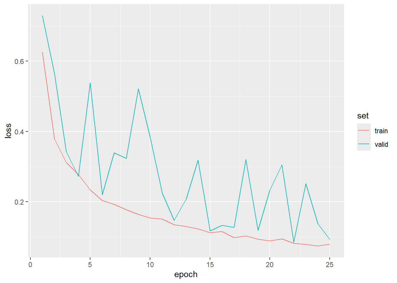
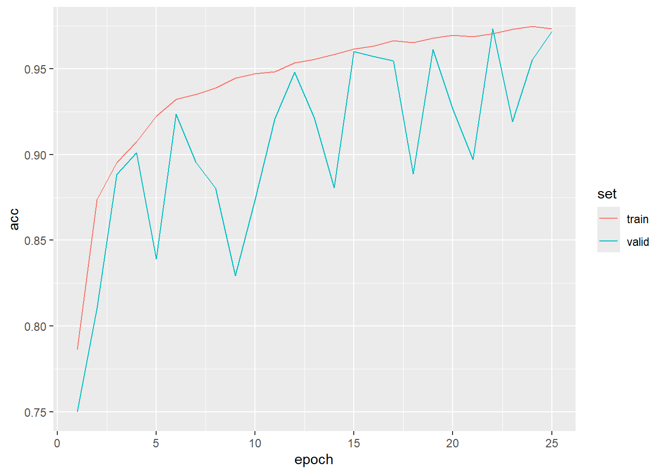
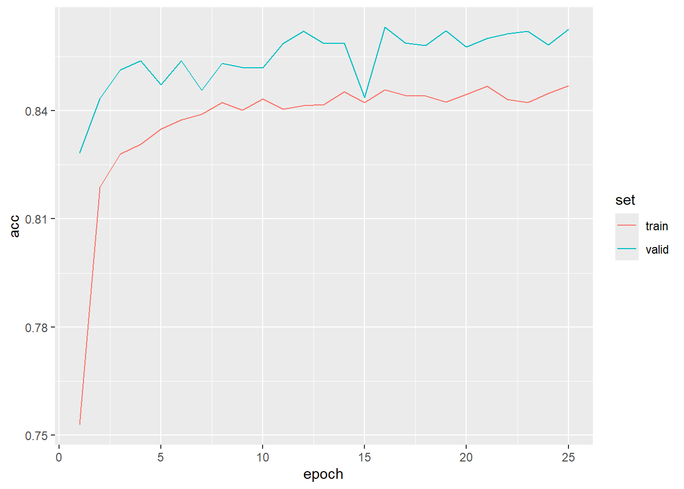
To begin exploring the results, we first load the saved model using luz_load() and the training logs using read_csv(). We then plot the logs using ggplot2. As is common, the validation loss and overall accuracy were noisier than those for the training data. However, it is clear that the model improved its performance over the training epochs, and their is no indication of overfitting.
12.4.3.2 Validate on Test Data
We now assess the model using the withheld test data. We first perform predictions on the withheld test data, move the results to the CPU, extract the index for the class that has the highest predicted logit, and convert the result to a base R array. Both the results are the associated reference labels are converted from numeric codes to class names using the forcats package and the recode() function. Lastly, the predictions and reference labels are merged to a single data frame, and the yardstick package is used to calculate assessment metrics.
The overall accuracy was 0.970 while the macro-averaged, class aggregated F1-score was 0.968. This indicates that more than 95% of the withheld test images were correctly labeled. This is higher than the results we obtained in the last section where the overall accuracy was 0.869 and the macro-averaged F1-score was 0.858. This generally suggests that incorporating convolution and the entire image as opposed to aggregating the images to channel means improved performance. This highlights the value of convolutional neural networks: being able to model spatial context information is of great value for performing scene labeling or classification tasks.
predTest <- predict(cnnModel, testDL)$detach()$to(device="cpu")
predTest <- predTest |>
  torch_argmax(dim=2) |>
  as.array(predTest)
truth <- testDF$Label + 1truth <- as.factor(truth) |>
fct_recode("AnnualCrop" = "1",
"Forest" = "2",
"HerbaceousVegetation" = "3",
"Highway" = "4",
"Industrial" = "5",
"Pasture" = "6",
"PermanentCrop" = "7",
"Residential" = "8",
"River" = "9",
"SeaLake" = "10") predTest <- as.factor(predTest) |>
fct_recode("AnnualCrop" = "1",
"Forest" = "2",
"HerbaceousVegetation" = "3",
"Highway" = "4",
"Industrial" = "5",
"Pasture" = "6",
"PermanentCrop" = "7",
"Residential" = "8",
"River" = "9",
"SeaLake" = "10") resultsDF <- data.frame(truth=truth,
pred=predTest)
accuracy(resultsDF,
truth=truth,
estimate=pred)$.estimate[1] 0.9702791recall(resultsDF,
truth=truth,
estimate=pred,
estimator="macro")$.estimate[1] 0.9684548precision(resultsDF,
truth=truth,
estimate=pred,
estimator="macro")$.estimate[1] 0.9691908f_meas(resultsDF,
truth=truth,
estimate=pred,
estimator="macro")$.estimate[1] 0.9685951conf_mat(resultsDF,
truth=truth,
estimate=pred) Truth
Prediction AnnualCrop Forest HerbaceousVegetation Highway
AnnualCrop 285 0 1 3
Forest 0 299 1 0
HerbaceousVegetation 1 0 289 1
Highway 1 0 0 230
Industrial 1 0 1 3
Pasture 2 1 1 0
PermanentCrop 10 0 7 5
Residential 0 0 0 2
River 0 0 0 6
SeaLake 0 0 0 0
Truth
Prediction Industrial Pasture PermanentCrop Residential River
AnnualCrop 0 3 4 0 0
Forest 0 2 0 0 0
HerbaceousVegetation 3 4 6 1 0
Highway 0 0 0 1 0
Industrial 244 0 0 2 0
Pasture 0 190 3 0 0
PermanentCrop 2 0 237 1 0
Residential 1 0 0 295 0
River 0 1 0 0 250
SeaLake 0 0 0 0 0
Truth
Prediction SeaLake
AnnualCrop 0
Forest 0
HerbaceousVegetation 0
Highway 0
Industrial 0
Pasture 0
PermanentCrop 0
Residential 0
River 1
SeaLake 358Lastly, we generated some chance-adjusted agreement measures along with their non-adjusted counterparts using the mice() function from micer.
mice(resultsDF$truth,
resultsDF$pred,
mappings=levels(as.factor(resultsDF$truth)),
multiclass = TRUE)$Mappings
[1] "AnnualCrop" "Forest" "HerbaceousVegetation"
[4] "Highway" "Industrial" "Pasture"
[7] "PermanentCrop" "Residential" "River"
[10] "SeaLake"
$confusionMatrix
Reference
Predicted AnnualCrop Forest HerbaceousVegetation Highway
AnnualCrop 285 0 1 3
Forest 0 299 1 0
HerbaceousVegetation 1 0 289 1
Highway 1 0 0 230
Industrial 1 0 1 3
Pasture 2 1 1 0
PermanentCrop 10 0 7 5
Residential 0 0 0 2
River 0 0 0 6
SeaLake 0 0 0 0
Reference
Predicted Industrial Pasture PermanentCrop Residential River
AnnualCrop 0 3 4 0 0
Forest 0 2 0 0 0
HerbaceousVegetation 3 4 6 1 0
Highway 0 0 0 1 0
Industrial 244 0 0 2 0
Pasture 0 190 3 0 0
PermanentCrop 2 0 237 1 0
Residential 1 0 0 295 0
River 0 1 0 0 250
SeaLake 0 0 0 0 0
Reference
Predicted SeaLake
AnnualCrop 0
Forest 0
HerbaceousVegetation 0
Highway 0
Industrial 0
Pasture 0
PermanentCrop 0
Residential 0
River 1
SeaLake 358
$referenceCounts
AnnualCrop Forest HerbaceousVegetation
300 300 300
Highway Industrial Pasture
250 250 200
PermanentCrop Residential River
250 300 250
SeaLake
359
$predictionCounts
AnnualCrop Forest HerbaceousVegetation
296 302 305
Highway Industrial Pasture
232 251 197
PermanentCrop Residential River
262 298 258
SeaLake
358
$overallAccuracy
[1] 0.9702791
$MICE
[1] 0.9668906
$usersAccuracies
AnnualCrop Forest HerbaceousVegetation
0.9628378 0.9900662 0.9475410
Highway Industrial Pasture
0.9913793 0.9721115 0.9644670
PermanentCrop Residential River
0.9045801 0.9899329 0.9689922
SeaLake
1.0000000
$CTBICEs
AnnualCrop Forest HerbaceousVegetation
0.9583035 0.9888541 0.9411402
Highway Industrial Pasture
0.9905202 0.9693323 0.9616894
PermanentCrop Residential River
0.8950712 0.9887045 0.9659022
SeaLake
1.0000000
$producersAccuracies
AnnualCrop Forest HerbaceousVegetation
0.9500000 0.9966666 0.9633333
Highway Industrial Pasture
0.9200000 0.9760000 0.9500000
PermanentCrop Residential River
0.9480000 0.9833333 1.0000000
SeaLake
0.9972145
$RTBICEs
AnnualCrop Forest HerbaceousVegetation
0.9438993 0.9962599 0.9588595
Highway Industrial Pasture
0.9120277 0.9736083 0.9460916
PermanentCrop Residential River
0.9428180 0.9812997 1.0000000
SeaLake
0.9967977
$f1Scores
AnnualCrop Forest HerbaceousVegetation
0.9563758 0.9933554 0.9553719
Highway Industrial Pasture
0.9543568 0.9740519 0.9571788
PermanentCrop Residential River
0.9257812 0.9866220 0.9842519
SeaLake
0.9986053
$f1Efficacies
AnnualCrop Forest HerbaceousVegetation
0.9510469 0.9925432 0.9499172
Highway Industrial Pasture
0.9496548 0.9714656 0.9538268
PermanentCrop Residential River
0.9183244 0.9849882 0.9826554
SeaLake
0.9983963
$macroPA
[1] 0.9684547
$macroRTBUCE
[1] 0.9651662
$macroUA
[1] 0.9691908
$macroCTBICE
[1] 0.9659518
$macroF1
[1] 0.9688226
$macroF1Efficacy
[1] 0.965558812.5 ResNet-32
There are a variety of scene labeling CNN architectures, and many of these architectures have been trained using large datasets, such as ImageNet. This provides an opportunity to implement transfer learning where the model is initialized using parameters learned from a different problem. The model can then be trained starting from these initial weights as opposed to being trained from a random initiation. It is also possible to only train portions of the model, such as just the fully connected component.
In this second example, we train a ResNet-32 architecture for the EuroSAT problem. ImageNet-based weights are loaded, the CNN component is frozen, and only the fully connected component is trained.
12.5.1 Define Model
We generate the ResNet-32 model using a version provided by the torchvision package. As normal, this is conducted by subclassing nn_module(). We are allowing the user to specify the number of output classes, whether or not to load pre-trained, ImageNet-based weights, and whether or not to train the CNN component of the model. If trainCNN=TRUE it will be trainable during the learning process. If trainCNN=FALSE it will not be trainable.
An if statement and a for loop over the model parameters are used to set the requires_grad_ property for parameters. If this is set to FALSE for a parameter, it will not be trainable during the learning process.
Next, we replace the final fully connected component with a new fully connected component that accepts the number of input features from the prior layer in the ResNet-32 architecture and generates the desired number of class logits. This is necessary since the number of classes in the ImageNet dataset is different from that in the EuroSat dataset. It is important that this is done after setting trainable parameters as not trainable since we always want to train this component of the model. The default behavior is for components to be trainable, so replacing the original fully connected layer with a new one makes the component trainable.
resNet32 <- nn_module(
"convnet",
initialize = function(outCls, pretrained, trainCNN){
self$outCls <- outCls
self$pretrained <- pretrained
self$trainCNN <- trainCNN
self$model <- torchvision::model_resnet34(pretrained=self$pretrained)
if(self$trainCNN == FALSE){
for(par in self$parameters){
par$requires_grad_(FALSE)
}
}
self$model$fc <- nn_linear(self$model$fc$in_features, self$outCls)
},
forward = function(x) {
x <- self$model(x)
return(x)
}
)12.5.2 Define Dataset Subclass
We also need to edit our dataset subclass. Since we plan to use ImageNet weights, we will only use the red, green, and blue channels, since ImageNet data only have these channels. We also normalize the channels relative to the published ImageNet band means and standard deviations. This is generally recommended when initializing using ImageNet weights and using transfer learning. This is accomplished using transform_normalize() from torchvision. We have also removed the division by 10,000 step since the normalization makes this unnecessary. Next, we re-instantiate the datasets and dataloaders using the new dataset subclass.
eurosatDataSet <- torch::dataset(
name = "eurosatDataSet",
initialize = function(df,
pth,
doAugs=FALSE){
self$df <- df
self$pth <- pth
self$doAugs <- doAugs
},
.getitem = function(i){
imgName <- unlist(self$df[i, "Filename"], use.names=FALSE)
label <- unlist(self$df[i, "Label"], use.names=FALSE) |>
torch_tensor(dtype=torch_int64()) |>
torch_add(1)
label <- label$squeeze()
label <- label |> torch_tensor(dtype=torch_int64())
img <- rast(paste0(self$pth, imgName)) |>
terra::subset(c(2,3,4)) |>
as.array() |>
torch_tensor(dtype=torch_float32())
img <- img$permute(c(3,2,1))
img <- torchvision::transform_normalize(img,
mean=c(0.406, 0.456, 0.485),
std=c(0.225, 0.224, 0.229))
if(self$doAugs == TRUE){
img <- torchvision::transform_random_horizontal_flip(img, p=0.5)
img <- torchvision::transform_random_vertical_flip(img, p=0.5)
}
return(list(preds = img, label = label))
},
.length = function(){
return(nrow(self$df))
}
)trainDS <- eurosatDataSet(df=trainDF,
pth=fldPth,
doAugs=TRUE)
valDS <- eurosatDataSet(df=valDF,
pth=fldPth,
doAugs=TRUE)
testDS <- eurosatDataSet(df=testDF,
pth=fldPth,
doAugs=TRUE)trainDL <- torch::dataloader(trainDS,
batch_size=32,
shuffle=TRUE,
drop_last = TRUE)
valDL <- torch::dataloader(valDS,
batch_size=32,
shuffle=FALSE,
drop_last = TRUE)
testDL <- torch::dataloader(testDS,
batch_size=32,
shuffle=FALSE,
drop_last = FALSE)12.5.3 Fit Model with luz
Now that the data and model architecture are prepared, we can run the training process using luz. This is the same as the training process used above other than using the new architecture and training and validation dataloaders and changing the name of the saved logs and final model. As configured, ImageNet pre-trained weights are loaded (pretained=TRUE), and only the fully connected component of the architecture is trainable (trainCNN=FALSE). The training process will execute for 25 epochs, and the model parameters after the epoch with the lowest validation set loss will be saved as the final model.
If you choose to run the training loop, it will take several hours to execute. We have provided a trained model file if you want to execute later code in this chapter without training the model from scratch.
fitted <- resNet32 |>
setup(
loss = nn_cross_entropy_loss(),
optimizer = optim_adam,
metrics=luz_metric_accuracy()
) |>
set_hparams(
outCls=10,
pretrained=TRUE,
trainCNN=FALSE
) |>
fit(data = trainDL,
epochs = 25,
valid_data = valDL,
callbacks = list(luz_callback_csv_logger("gslrData/chpt12/output/resnetLogs.csv"),
luz_callback_keep_best_model(monitor = "valid_loss",
mode = "min",
min_delta = 0)),
accelerator = accelerator(device_placement = TRUE,
cpu = FALSE,
cuda_index = torch::cuda_current_device()),
verbose=TRUE)
luz_save(fitted, "gslrData/chpt12/output/resnetModel.pt")12.5.4 Validate Model
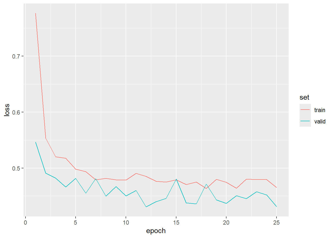
The validation process is the same as that used above and has been provided below. We did not obtain the same level of accuracy that we did for our original model. This may be because we only used the red, green, and blue bands. Also, the model parameters learned for the ImageNet problem may have been sub-optimal for this task. It would be interesting to train the ResNet-32 architecture without freezing the CNN component. It would also be interesting to augment the architecture to accept all ten image bands.
predTest <- predict(resnetModel, testDL)$detach()$to(device="cpu")
predTest <- predTest |>
torch_argmax(dim=2) |>
as.array(predTest)
truth <- testDF$Label + 1
truth <- as.factor(truth) |>
  fct_recode("AnnualCrop" = "1",
             "Forest" = "2",
             "HerbaceousVegetation" = "3",
             "Highway" = "4",
             "Industrial" = "5",
             "Pasture" = "6",
             "PermanentCrop" = "7",
             "Residential" = "8",
             "River" = "9",
             "SeaLake" = "10")
predTest <- as.factor(predTest) |>
  fct_recode("AnnualCrop" = "1",
             "Forest" = "2",
             "HerbaceousVegetation" = "3",
             "Highway" = "4",
             "Industrial" = "5",
             "Pasture" = "6",
             "PermanentCrop" = "7",
             "Residential" = "8",
             "River" = "9",
             "SeaLake" = "10")
resultsDF <- data.frame(truth=truth,
pred=predTest)
accuracy(resultsDF,
truth=truth,
estimate=pred)$.estimate[1] 0.8648061recall(resultsDF, truth=truth, estimate=pred, estimator="macro")$.estimate[1] 0.8558336precision(resultsDF, truth=truth, estimate=pred, estimator="macro")$.estimate[1] 0.8659689f_meas(resultsDF, truth=truth, estimate=pred, estimator="macro")$.estimate[1] 0.8589577conf_mat(resultsDF, truth=truth, estimate=pred) Truth
Prediction AnnualCrop Forest HerbaceousVegetation Highway
AnnualCrop 268 0 2 3
Forest 1 284 9 0
HerbaceousVegetation 4 4 256 5
Highway 5 2 8 204
Industrial 0 0 0 5
Pasture 5 1 2 0
PermanentCrop 12 0 11 8
Residential 0 1 8 1
River 5 1 3 24
SeaLake 0 7 1 0
Truth
Prediction Industrial Pasture PermanentCrop Residential River
AnnualCrop 0 0 11 1 3
Forest 0 10 0 0 0
HerbaceousVegetation 1 11 13 4 5
Highway 12 11 18 9 42
Industrial 216 0 1 3 4
Pasture 0 154 0 0 3
PermanentCrop 8 6 197 4 1
Residential 9 0 8 273 2
River 2 7 2 4 189
SeaLake 2 1 0 2 1
Truth
Prediction SeaLake
AnnualCrop 2
Forest 2
HerbaceousVegetation 1
Highway 4
Industrial 0
Pasture 1
PermanentCrop 0
Residential 0
River 4
SeaLake 345mice(resultsDF$truth,
resultsDF$pred,
mappings=levels(as.factor(resultsDF$truth)),
multiclass = TRUE)$Mappings
[1] "AnnualCrop" "Forest" "HerbaceousVegetation"
[4] "Highway" "Industrial" "Pasture"
[7] "PermanentCrop" "Residential" "River"
[10] "SeaLake"
$confusionMatrix
Reference
Predicted AnnualCrop Forest HerbaceousVegetation Highway
AnnualCrop 268 0 2 3
Forest 1 284 9 0
HerbaceousVegetation 4 4 256 5
Highway 5 2 8 204
Industrial 0 0 0 5
Pasture 5 1 2 0
PermanentCrop 12 0 11 8
Residential 0 1 8 1
River 5 1 3 24
SeaLake 0 7 1 0
Reference
Predicted Industrial Pasture PermanentCrop Residential River
AnnualCrop 0 0 11 1 3
Forest 0 10 0 0 0
HerbaceousVegetation 1 11 13 4 5
Highway 12 11 18 9 42
Industrial 216 0 1 3 4
Pasture 0 154 0 0 3
PermanentCrop 8 6 197 4 1
Residential 9 0 8 273 2
River 2 7 2 4 189
SeaLake 2 1 0 2 1
Reference
Predicted SeaLake
AnnualCrop 2
Forest 2
HerbaceousVegetation 1
Highway 4
Industrial 0
Pasture 1
PermanentCrop 0
Residential 0
River 4
SeaLake 345
$referenceCounts
AnnualCrop Forest HerbaceousVegetation
300 300 300
Highway Industrial Pasture
250 250 200
PermanentCrop Residential River
250 300 250
SeaLake
359
$predictionCounts
AnnualCrop Forest HerbaceousVegetation
290 306 304
Highway Industrial Pasture
315 229 166
PermanentCrop Residential River
247 302 241
SeaLake
359
$overallAccuracy
[1] 0.8648061
$MICE
[1] 0.8493927
$usersAccuracies
AnnualCrop Forest HerbaceousVegetation
0.9241379 0.9281045 0.8421052
Highway Industrial Pasture
0.6476190 0.9432314 0.9277108
PermanentCrop Residential River
0.7975708 0.9039735 0.7842323
SeaLake
0.9610028
$CTBICEs
AnnualCrop Forest HerbaceousVegetation
0.9148817 0.9193323 0.8228400
Highway Industrial Pasture
0.6125031 0.9375742 0.9220601
PermanentCrop Residential River
0.7773981 0.8922570 0.7627304
SeaLake
0.9551689
$producersAccuracies
AnnualCrop Forest HerbaceousVegetation
0.8933333 0.9466666 0.8533333
Highway Industrial Pasture
0.8160000 0.8640000 0.7700000
PermanentCrop Residential River
0.7880000 0.9100000 0.7560000
SeaLake
0.9610028
$RTBICEs
AnnualCrop Forest HerbaceousVegetation
0.8803185 0.9401592 0.8354380
Highway Industrial Pasture
0.7976637 0.8504471 0.7520215
PermanentCrop Residential River
0.7668734 0.8990188 0.7316845
SeaLake
0.9551689
$f1Scores
AnnualCrop Forest HerbaceousVegetation
0.9084745 0.9372937 0.8476821
Highway Industrial Pasture
0.7221239 0.9018789 0.8415300
PermanentCrop Residential River
0.7927565 0.9069767 0.7698574
SeaLake
0.9610028
$f1Efficacies
AnnualCrop Forest HerbaceousVegetation
0.8972674 0.9296292 0.8290911
Highway Industrial Pasture
0.6929272 0.8918879 0.8284053
PermanentCrop Residential River
0.7720999 0.8956251 0.7468850
SeaLake
0.9551689
$macroPA
[1] 0.8558336
$macroRTBUCE
[1] 0.8408794
$macroUA
[1] 0.8659688
$macroCTBICE
[1] 0.8516746
$macroF1
[1] 0.8608714
$macroF1Efficacy
[1] 0.846242512.6 Concluding Remarks
We have now discussed how to use fully connected and CNN architectures for scene labeling tasks where the entire image extent is assigned to a single label. In the next chapter, we explore means to potentially improve model performance. The remaining chapters in this section explore semantic segmentation where each pixel is labeled separately.
12.7 Questions
- Explain the purpose of padding when performing convolution operations.
- In order to reduce the size of an array in the spatial dimensions, it is common to use max pooling. How could downsizing be accomplished using a convolutional layer instead?
- A convolutional layer accepts 18 feature maps and generates 50 feature maps. It uses a kernel size of 3x3. How many weight and bias terms are associated with this layer?
- The convolutional layer from Question 3 is followed by a batch normalization layer. How many scale and shift parameters will this layer have?
- Why is it necessary to flatten tensors to a 1D vector prior to passing the data to the first fully connected layer in the architecture?
- What is the purpose of the
forward()method within ann_module()subclass? - Explain how the input data and input label tensor shapes are similar and different for a fully connected vs. CNN architecture.
- Explain the concept of a residual connection, such as those used within ResNet architectures.
12.8 Exercises
Task 1
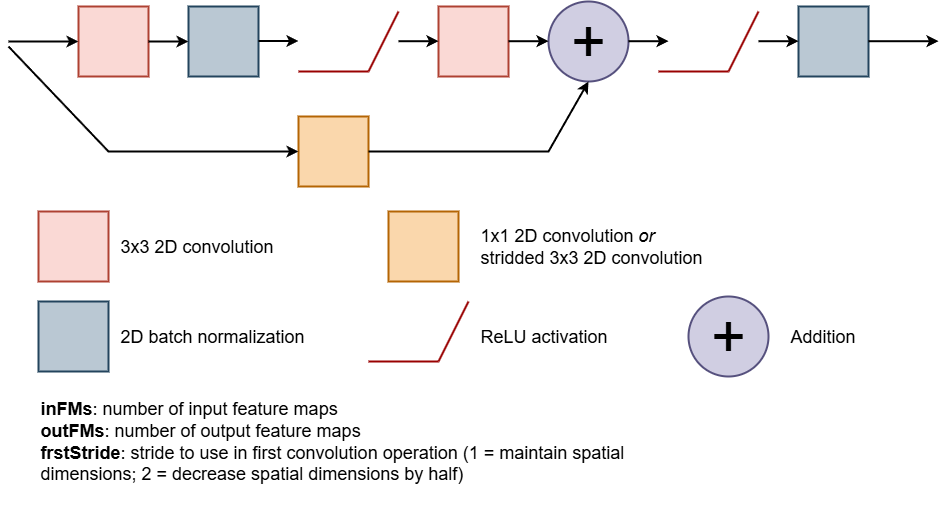
Subclass nn_module() to create a residual block, as implemented in the ResNet architectures. This block is conceptualized below. The user should be able to specify the number of input feature maps (inFMs), the number of output feature maps (outFMs), and the stride to use with the 2D convolution operation (frstStride). The first convolution block must accept the number of input feature maps and generate the desired number of output feature maps. The second convolutional block along the main path must accept the number of output feature maps from the first convolution block and maintain the number of feature maps. The processing that occurs along the residual connection will vary as follows:
- If the first convolution block uses a stride of 1 and the number of input feature maps and output feature maps are the same, no processing is required and an identity connection should be used where the input is added to the output of the second convolution block in the main path.
- If the first convolution block uses a stride of 1 and the number of input feature maps and output feature maps are different, a projection connection should be used where the number of feature maps is altered to match the number of output feature maps along the main path but the spatial dimensions are maintained using 1x1 2D convolution with a stride of 1 and padding of 0. This output should then be added to the output of the second convolution block in the main path.
- If the first convolution block uses a stride of 2 and the number of input feature maps and output feature maps are different, a projection connections should be used where the number of feature maps and the spatial dimensions are altered to match the number of output feature maps and spatial dimensions along the main path using 3x3 2D convolution with a stride of 2 and a padding of 2. This output should then be added to the output of the second convolution block in the main path.
As conceptualized in the diagram, you will also need to implement ReLU action functions and batch normalization. You may find it useful to do some background research on the residual blocks and the ResNet architecture prior to attempting this.
Once you have generated the architecture, instantiate it and test it on some random data of the correct shape.
Task 2
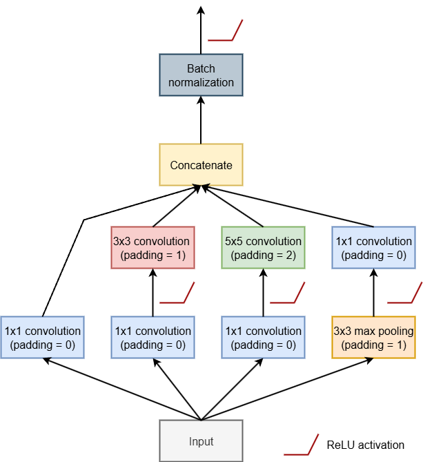
Generate a modified Inception block, inspired by the InceptionNet-family of architectures and as conceptualized in the diagram below, by subclass nn_module(), The goal of this block is to capture patterns at different spatial scales by processing the input data using different window sizes along different branches of the architecture. The feature maps generated by the different branches are then concatenated or stacked. Note that the spatial dimensions sizes should not change throughout the architecture. We have also noted where ReLU activation functions should be applied. You only need to apply batch normalization after the concatenation of the final set of feature maps. As with the residual block, doing some background research on InceptionNet and Inception blocks may be useful prior to attempting to generate the block.
Once you have generated the architecture, instantiate it and test it on some random data of the correct shape.
Task 3
Depthwise separable convolution is a common component of efficient CNN architectures, such as those from the MobileNet family. This process consists of two components: depthwise convolution and pointwise convolution. In contrast to traditional convolution blocks, depthwise convolution learns separate feature maps for each input feature map, as opposed to applying all learned feature maps to every input feature map. The results are then concatenated or stacked and passed to a pointwise convolution layer where the output of depthwise component is further processed. Depthwise convolution is generally implemented using 3x3 2D convolution. If the groups parameter is set to the number of input feature maps then a separate kernel is learned for each input feature map. If groups = 1, then all learned feature maps are applied to all inputs, which is equivalent to traditional 2D convolution. Pointwise convolution is implemented using 1x1 2D convolution with a stride and padding of 1. This step essentially performs feature reduction on the concatenated stack of feature maps.
Create a depthwise separable convolution block by subclassing nn_module(). The user should be able to specify the number of input feature maps and the number of output feature maps. Following pointwise convolution, apply batch normalization followed by a ReLU activation function. As with the prior two tasks, doing some background research on depthwise separable convolution may be useful prior to attempting to generate the block.
Once you have generated the architecture, instantiate it and test it on some random data of the correct shape.
