2 Imagery and Digital Terrain Data
2.1 Topics Covered
- Band ratios from multispectral imagery
- Tasseled cap transformation
- Principal component analysis (PCA) on raster data for feature reduction
- Spatial enhancement via convolution filters
- Land surface parameters (LSPs) from a digital terrain model (DTM)
- Customizing moving windows
2.2 Introduction
Continuing from the last chapter, we now explore means to create derived products from image bands and digital terrain models (DTMs). For multispectral image data, we explore normalized difference band ratios, the tasseled cap transformation, principal component analysis (PCA), and convolution. For DTMs, we explore creating a wide variety of land surface parameters (LSPs).
We primarily rely on the terra package; however, we also load in the tidyverse for general data manipulation and tmap and tmaptools for map creation and geospatial data visualization. Additional raster processing functionality is provided by RStoolbox, spatialEco, and MultiscaleDTM.
For our demonstrations, we use a Landsat 8 Operational Land Imager (OLI) scene from March of 2024 representing leaf-off conditions and a Landsat 9 Operational Land Imager-2 (OLI-2) scene from September of 2024 representing leaf-on conditions. The images cover the area around Philadelphia, Pennsylvania, USA. They are read in using the rast() from terra. The bands are renamed using names(), and the images are visualized using different band combinations and plotRGB(). Comparing the two images, difference in spectral reflectance between the leaf-on and leaf-off data are apparent.
folderPath <- "gslrData/chpt2/data/"

lOff <- rast(str_glue("{folderPath}ls8_3_11_2024_SR.tif"))
lOn <- rast(str_glue("{folderPath}ls9_9_11_2024_SR.tif"))

names(lOff) <- c("Edge",
                 "Blue",
                 "Green",
                 "Red",
                 "NIR",
                 "SWIR1",
                 "SWIR2")
names(lOn) <- c("Edge",
                "Blue",
                "Green",
                "Red",
                "NIR",
                "SWIR1",
                "SWIR2")

plotRGB(lOff, r=5, g=4, b=3, stretch="lin")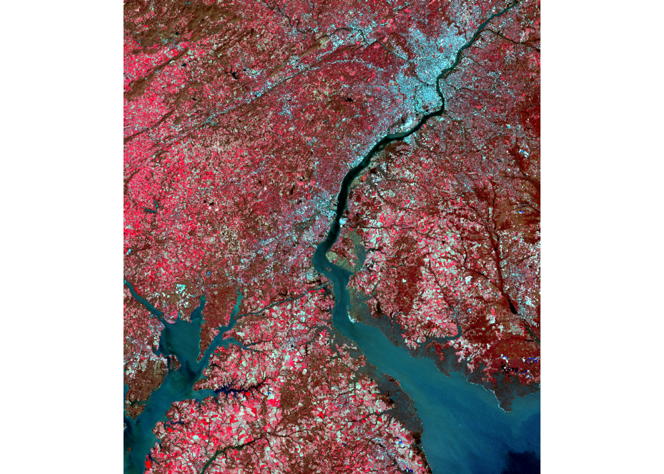
plotRGB(lOn, r=5, g=4, b=3, stretch="lin")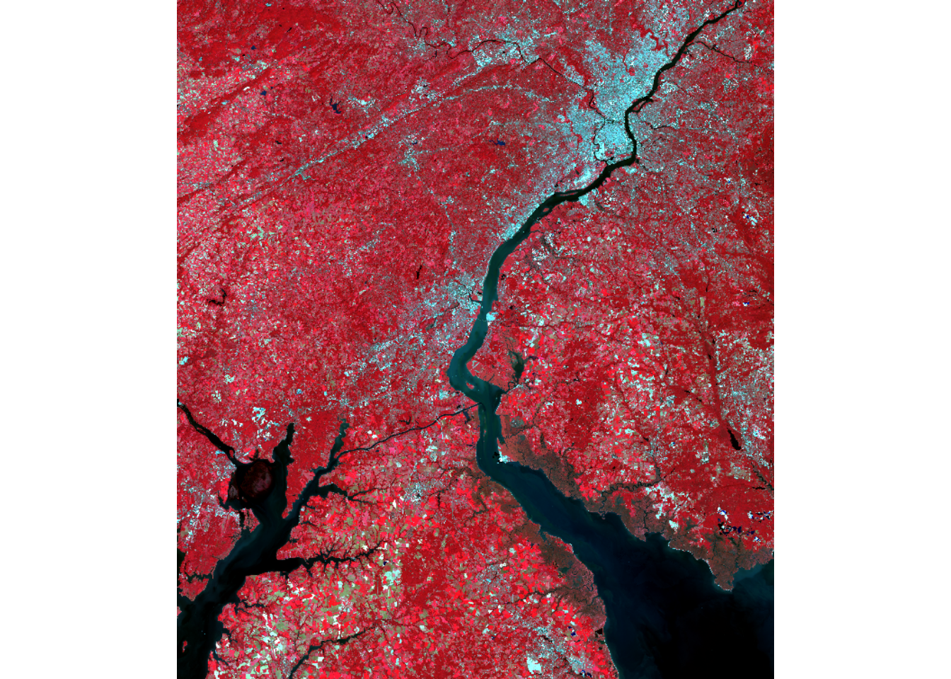
plotRGB(lOff, r=7, g=5, b=3, stretch="lin")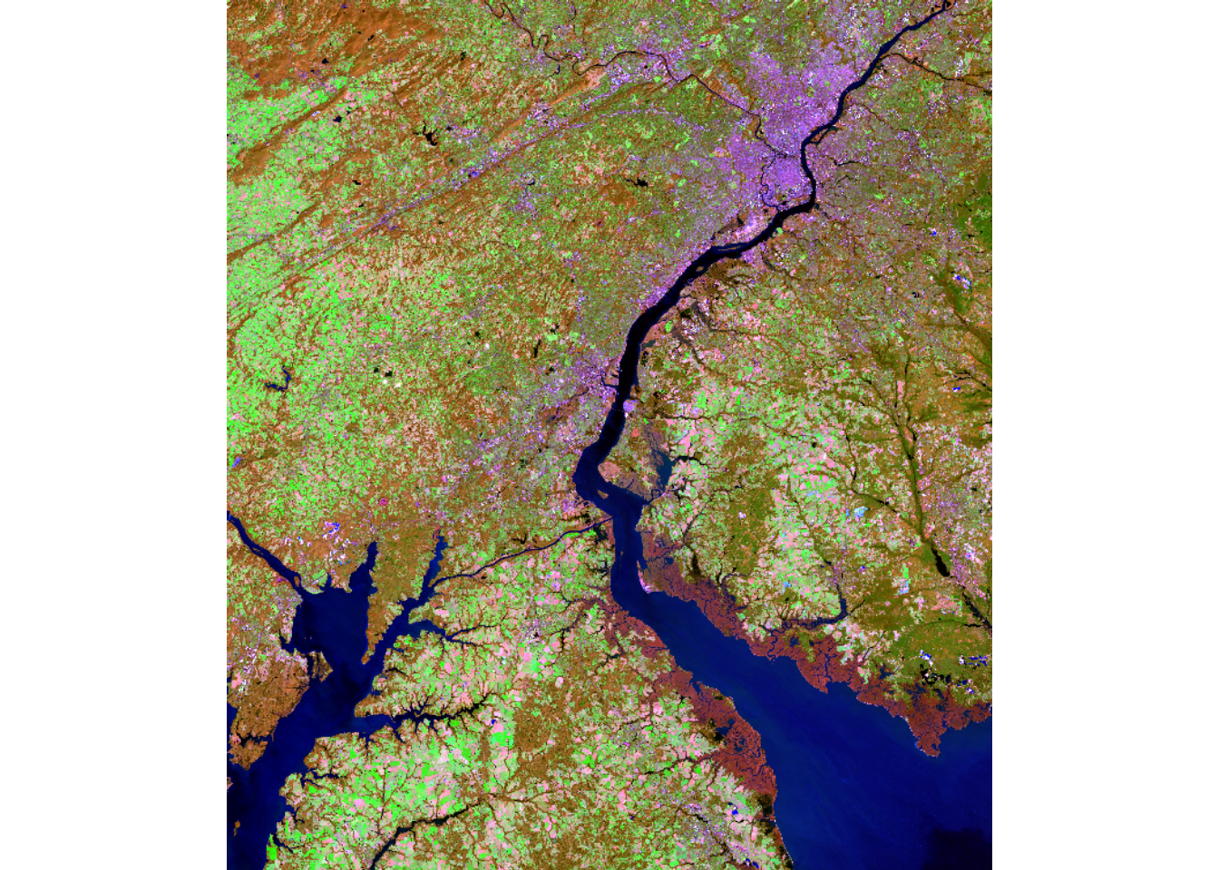
plotRGB(lOn, r=7, g=5, b=3, stretch="lin")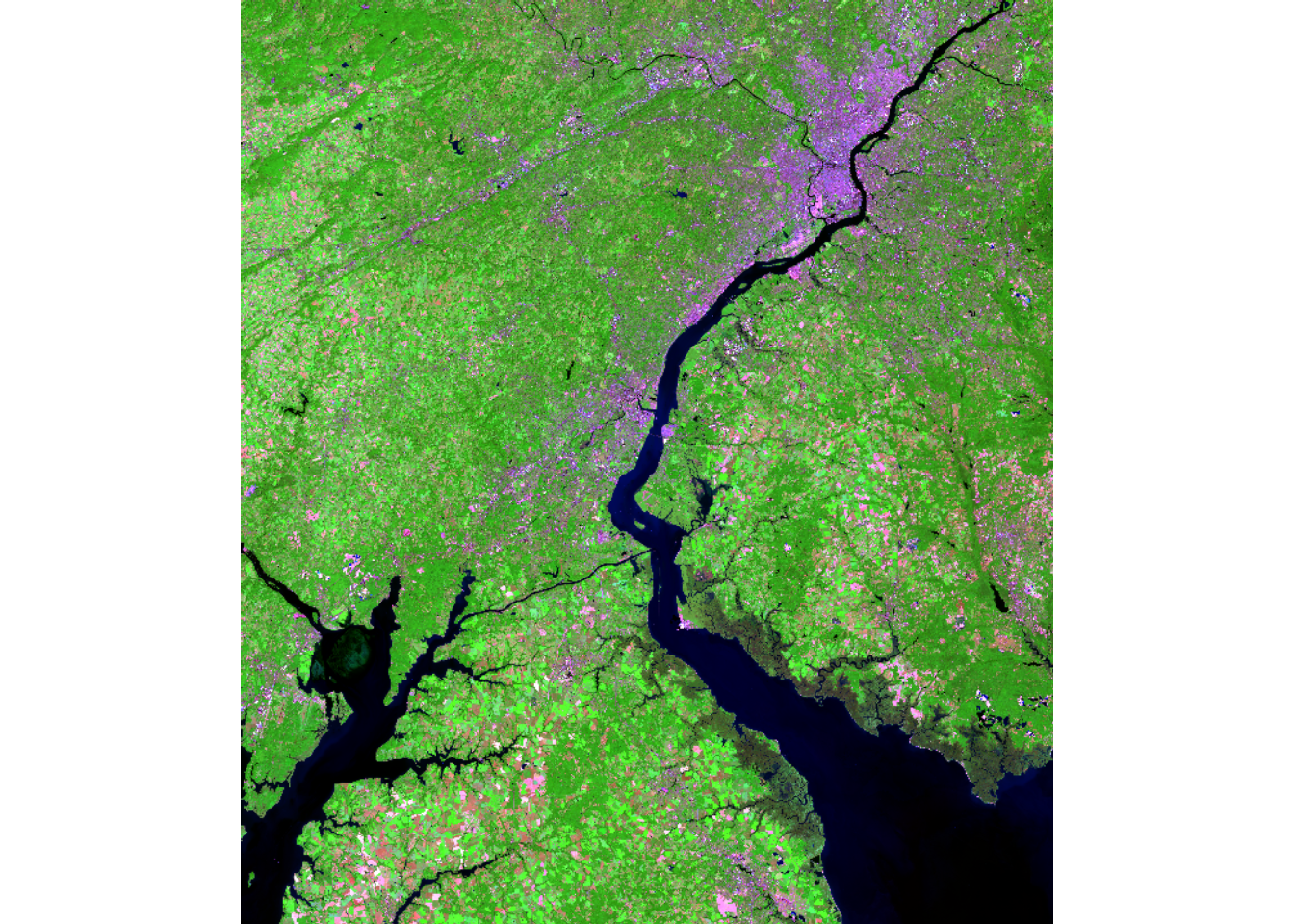
2.3 Image Processing
2.3.1 Band Ratios
Table 2.1 lists and describes some common band ratios calculated from multispectral satellite data, such as those from the Landsat and Sentinel-2 missions and associated sensors. In the following code blocks, we demonstrate calculating example ratios using raster math and terra.
| Band Ratio | Equation | Use |
|---|---|---|
| Normalized Difference Vegetation Index (NDVI) | (NIR-Red)/(NIR+Red) | Vegetation occurrence and health |
| Normalized Difference Built-Up Index (NDBI) | (SWIR-NIR)/(SWIR+NIR) | Ubanized areas; built-up areas; impervious surface |
| Normalized Difference Snow Index (NDSI) | (Green-SWIR)/(Green+SWIR) | Prescence of snow or ice |
| Normalized Difference Water Index (NDWI) after McFeeter | (Green-NIR)/(Green+NIR) | Presence of standing water |
| Normalized Difference Moisture Index (NDMI) | (NIR-SWIR)/(NIR_SWIR) | Vegetation water content |
In our first example, we calculate the normalized difference vegetation index (NDVI) for both the leaf-off and leaf-on data using the near infrared (NIR) and red channels. We visualize the resulting single-band raster grids using tmap.
Instead of saving the result to a new spatRaster object, the ratio could be added as a new channel to the image stack using c(). Since the ratio is derived from the input multispectral data, it will align with the input data had have the same extent and number of rows and columns of cells.
It is generally preferred to calculate band ratios using surface reflectance as opposed to digital number (DN) values.
ndviLOff <- (lOff$NIR-lOff$Red)/((lOff$NIR+lOff$Red)+.001)
ndviLOn <- (lOn$NIR-lOn$Red)/((lOn$NIR+lOn$Red)+.001)tm_shape(ndviLOff)+
tm_raster(col.scale = tm_scale_intervals(n=7,
style="quantile",
values = "brewer.greens"))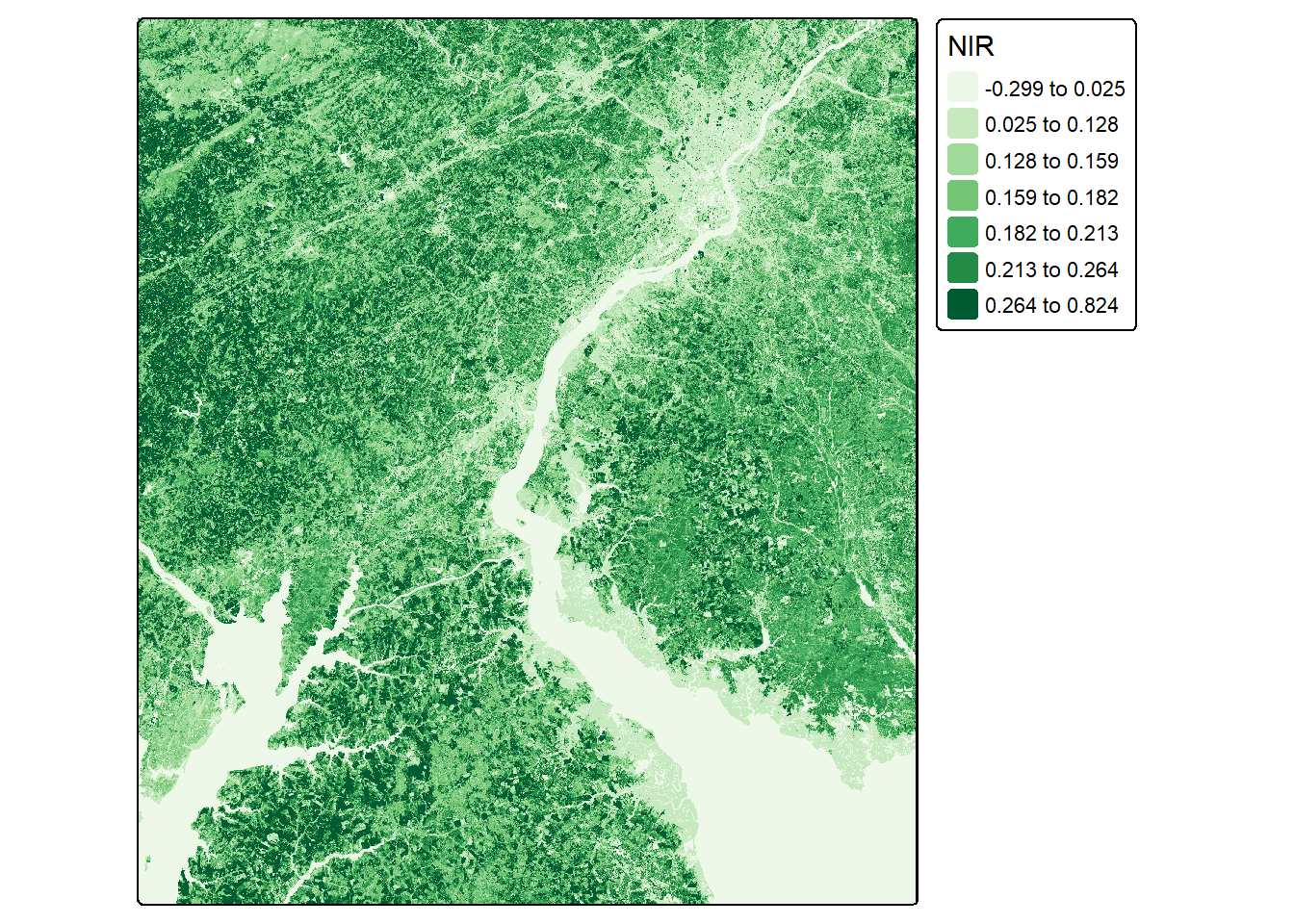
tm_shape(ndviLOn)+
  tm_raster(col.scale = tm_scale_intervals(n=7,
                                          style="quantile",
                                          values = "brewer.greens"))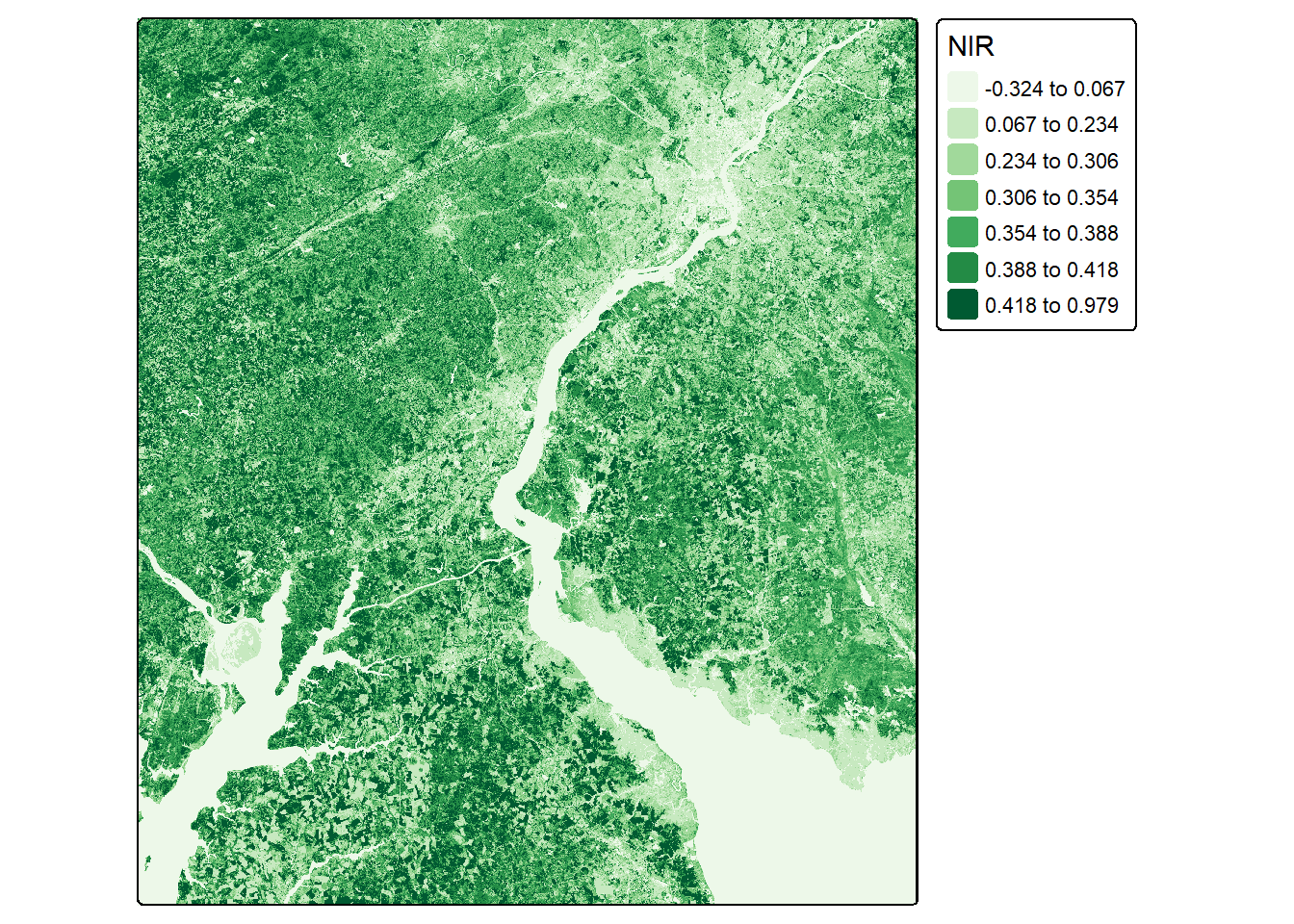
Other band ratios can be calculated using the same general method. In the next example, we calculate the normalized difference built-up index (NDBI) using the shortwave infrared 2 (SWIR2) and NIR bands. Next, we calculate a normalized difference water index (NDWI) using the green and NIR bands.
ndbiLOff <- (lOff$SWIR2-lOff$NIR)/((lOff$SWIR2+lOff$NIR)+.001)
ndbiLOn <- (lOn$SWIR2-lOn$NIR)/((lOn$SWIR2+lOn$NIR)+.001)tm_shape(ndbiLOff)+
tm_raster(col.scale = tm_scale_intervals(n=7,
style="quantile",
values = "brewer.reds"))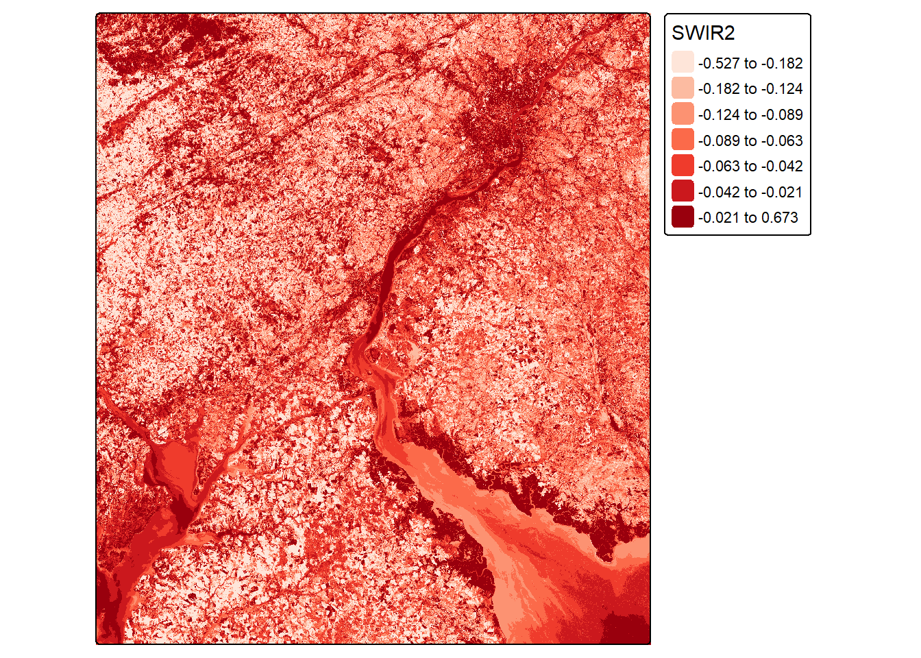
tm_shape(ndbiLOn)+
  tm_raster(col.scale = tm_scale_intervals(n=7,
                                          style="quantile",
                                          values = "brewer.reds"))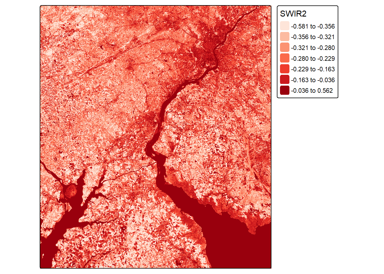
ndwiLOff <- (lOff$Green-lOff$NIR)/((lOff$Green+lOff$NIR)+.001)
ndwiLOn <- (lOn$Green-lOn$NIR)/((lOn$Green+lOn$NIR)+.001)tm_shape(ndwiLOff)+
tm_raster(col.scale = tm_scale_intervals(n=7,
style="quantile",
values = "brewer.blues"))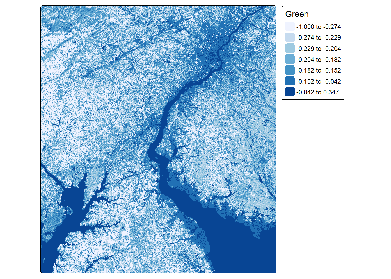
tm_shape(ndwiLOn)+
  tm_raster(col.scale = tm_scale_intervals(n=7,
                                          style="quantile",
                                          values = "brewer.blues"))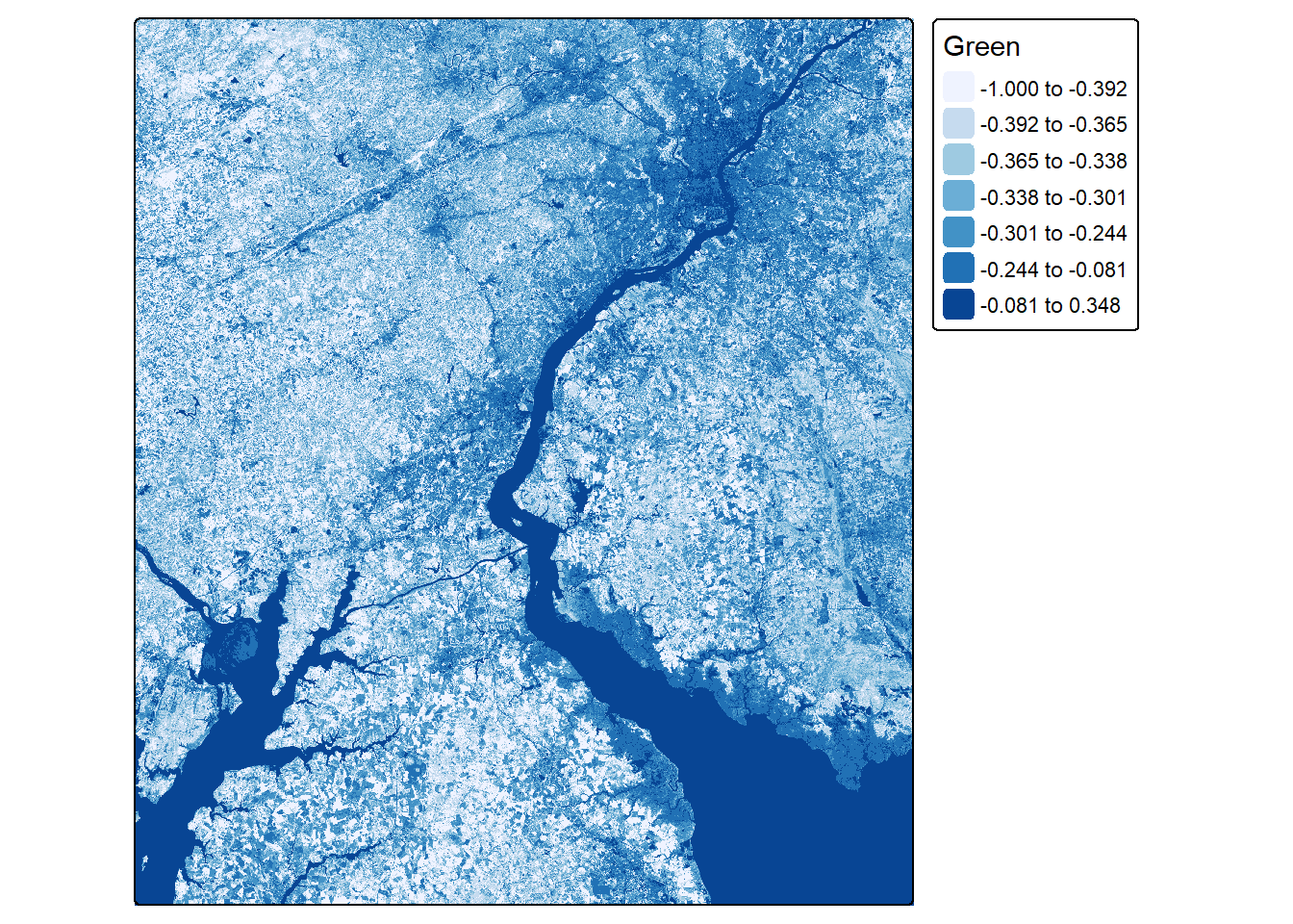
2.3.2 Tasseled Cap Transformation
The tasseled cap transformation is used to convert image bands into the following measures:
- Brightness: correlates with overall spectral brightness and soil brightness
- Greenness: correlates with the presence of photosynthetically active vegetation
- Wetness: correlates with the presence of standing water and water in soil and plant tissue
These measures are derived by multiplying the blue, green, red, NIR, SWIR1, and SWIR2 bands by pre-defined coefficients and summing the results. This transformation is commonly applied to Landsat Thematic Mapper (TM), Enhanced Thematic Mapper Plus (ETM+), OLI, or OLI-2 data. Coefficients have also been published for the Sentinel-2 Multispectral Instrument (MSI) sensor. The coefficients are generally meant to be applied to surface reflectance estimates as opposed to DN values.
Below, we use the published coefficients for the OLI and OLI-2 sensors to generate brightness, greenness, and wetness raster grids. We then merge the results to a single, multiband raster and display them using a false color composite. Areas with water generally show up as blue since wetness is mapped to the blue channel. Spectrally bright areas, such as impervious surfaces and bare soil, show up a red.
brightness <- 0.3029*lOff$Blue +
  0.2786*lOff$Green +
  0.4733*lOff$Red +
  0.5599*lOff$NIR +
  0.508*lOff$SWIR1 +
  0.1887*lOff$SWIR2

greenness <- -0.2951*lOff$Blue +
  -0.243*lOff$Green +
  -0.5424*lOff$Red +
  0.7276*lOff$NIR +
  0.0713*lOff$SWIR1 +
  -0.1608*lOff$SWIR2

wetness <- 0.1511*lOff$Blue +
  0.1973*lOff$Green +
  0.3283*lOff$Red +
  0.3407*lOff$NIR +
  -0.7117*lOff$SWIR1 +
  -0.4559*lOff$SWIR2

tcOff <- c(brightness, greenness, wetness)
plotRGB(tcOff, r=1, g=2, b=3, stretch="lin")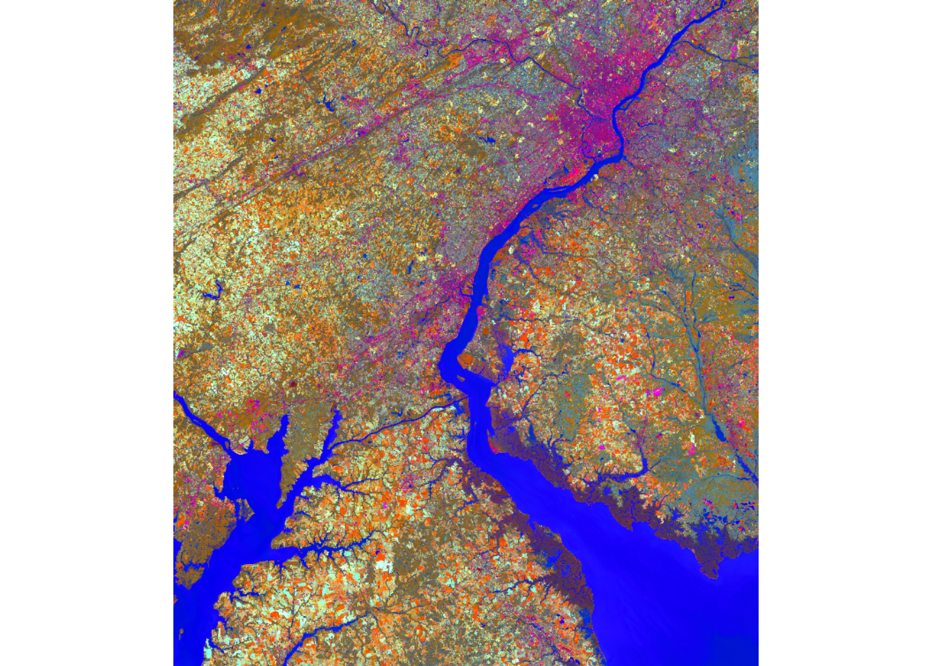
brightness <- 0.3029*lOn$Blue +
  0.2786*lOn$Green +
  0.4733*lOn$Red +
  0.5599*lOn$NIR +
  0.508*lOn$SWIR1 +
  0.1887*lOn$SWIR2

greenness <- -0.2951*lOn$Blue +
  -0.243*lOn$Green +
  -0.5424*lOn$Red +
  0.7276*lOn$NIR +
  0.0713*lOn$SWIR1 +
  -0.1608*lOn$SWIR2

wetness <- 0.1511*lOn$Blue +
  0.1973*lOn$Green +
  0.3283*lOn$Red +
  0.3407*lOn$NIR +
  -0.7117*lOn$SWIR1 +
  -0.4559*lOn$SWIR2

tcOn <- c(brightness, greenness, wetness)
plotRGB(tcOn, r=1, g=2, b=3, stretch="lin")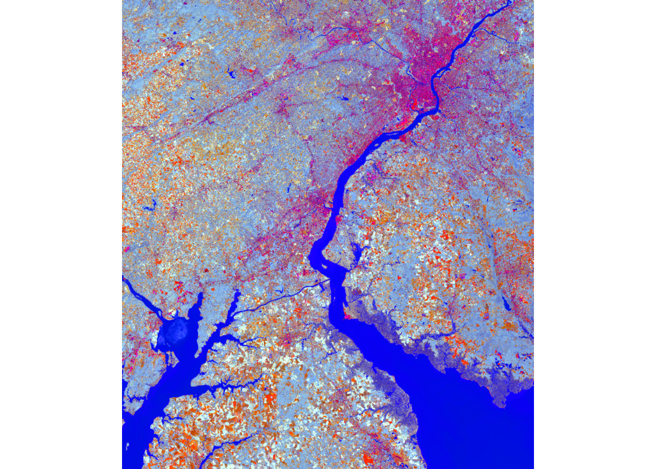
2.3.3 Principal Component Analysis
We explore the application of principal component analysis (PCA) to tabulated data in the next chapter. Here, it is applied to multiband raster data using the rasterPCA() function from the RStoolbox package. We first read in the leaf-on and leaf-off data again, rename the bands, then stack the two images into a single spatRaster object. We then perform the PCA to extract 14 components. Remember that the goal of PCA is to create linearly decorrelated data from the original, correlated image bands. The underlying idea is that variance equals information, so capturing the variance in the input data using a smaller number of bands results in feature reduction while maintaining the information content in the original image bands.
lOff <- rast(str_glue("{folderPath}ls8_3_11_2024_SR.tif"))
lOn <- rast(str_glue("{folderPath}ls9_9_11_2024_SR.tif"))

names(lOff) <- c("off_Edge",
                 "off_Blue",
                 "off_Green",
                 "off_Red",
                 "off_NIR",
                 "off_SWIR1",
                 "off_SWIR2")

names(lOn) <- c("on_Edge",
                "on_Blue",
                "on_Green",
                "on_Red",
                "on_NIR",
                "on_SWIR1",
                "on_SWIR2")

allBands <- c(lOff, lOn)

pcaOut <- rasterPCA(allBands, nSamples = NULL, nComp = 14, spca = FALSE)
Once the PCA data are generated, we can visualize the result as a false color composite. In our example, we use the first three principal component bands. The rasterPCA() function returns a list object where the PCA image is stored as a spatRaster in the map object.
plotRGB(pcaOut$map, r=1, b=2, g=3, stretch="lin")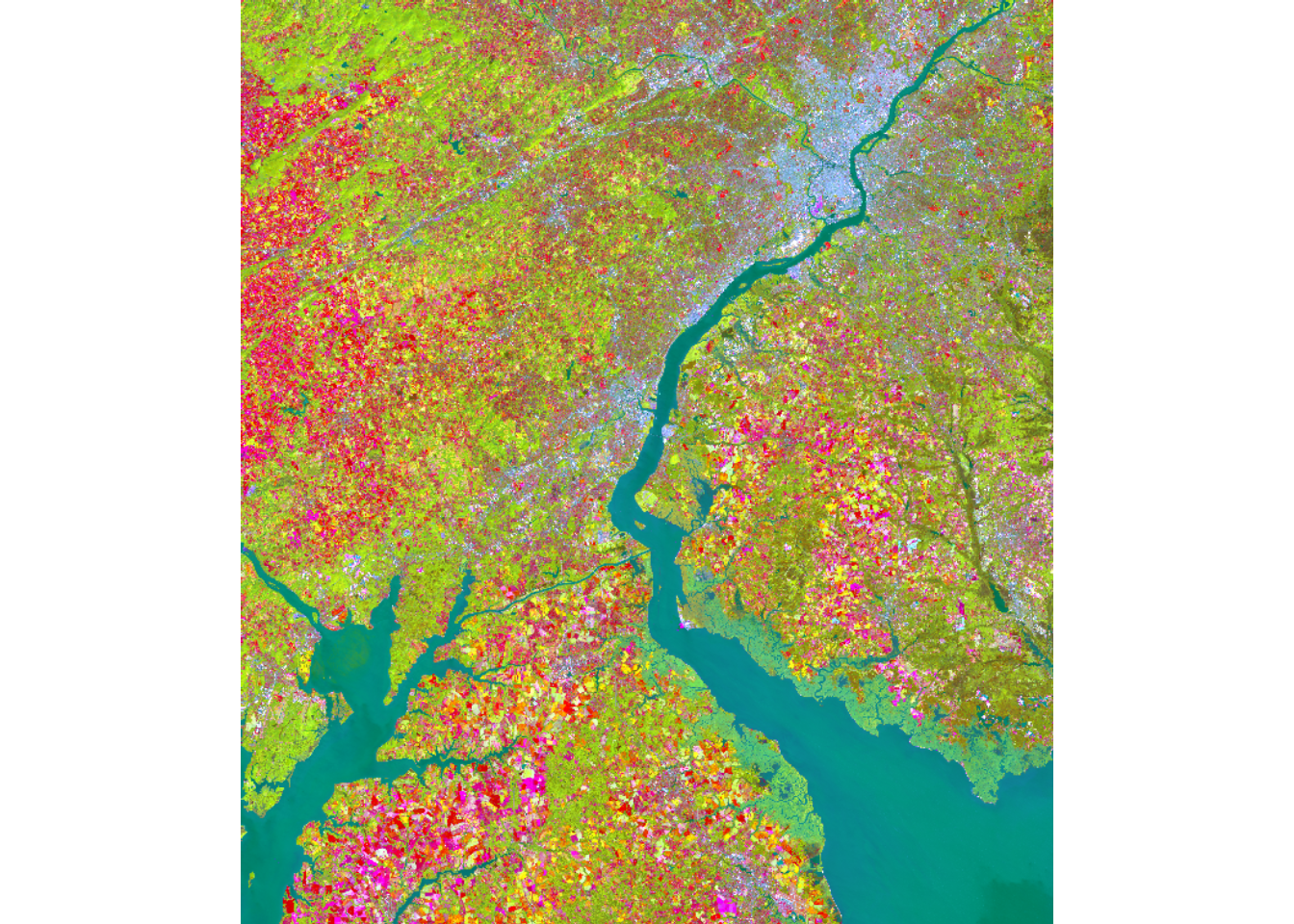
We can obtain PCA eigenvalues from the model object stored within the list object created by rasterPCA(). Larger values indicate more variance explained. By dividing the eigenvalue for a specific PCA band by the sum of all eigenvalues, we can obtain the percent of variance explained by that principal component. The results suggest that component one captures ~40% of the total variance in the data while component two captures ~18.5%. The first six principal components collectively capture ~91% of the variance from the original bands.
pcaOut$modelCall:
princomp(cor = spca, covmat = covMat)
Standard deviations:
Comp.1 Comp.2 Comp.3 Comp.4 Comp.5 Comp.6 Comp.7
7114.87746 3297.11634 2017.43885 1603.42419 1499.60854 622.83532 445.30067
Comp.8 Comp.9 Comp.10 Comp.11 Comp.12 Comp.13 Comp.14
364.26454 257.78072 186.06735 149.72014 109.27942 70.31829 56.08057
14 variables and 14108647 observations.pcaOut$model$sdev/(sum(pcaOut$model$sdev)) Comp.1 Comp.2 Comp.3 Comp.4 Comp.5 Comp.6
0.399844471 0.185292543 0.113376762 0.090109816 0.084275546 0.035002326
Comp.7 Comp.8 Comp.9 Comp.10 Comp.11 Comp.12
0.025025169 0.020471071 0.014486855 0.010456681 0.008414027 0.006141325
Comp.13 Comp.14
0.003951773 0.003151636 Comp.1 Comp.2 Comp.3 Comp.4 Comp.5 Comp.6 Comp.7 Comp.8
0.3998445 0.5851370 0.6985138 0.7886236 0.8728991 0.9079015 0.9329266 0.9533977
Comp.9 Comp.10 Comp.11 Comp.12 Comp.13 Comp.14
0.9678846 0.9783412 0.9867553 0.9928966 0.9968484 1.0000000 The loadings or eigenvectors are the coefficients that each band must be multiplied by in order to obtain each principal component. There are unique eigenvectors for each component and band combination. Eigenvectors serve a similar purpose as the coefficients used in the tasseled cap transformation demonstrated above: they allow for transforming the original bands into the new PC bands.
pcaOut$model$loadings
Loadings:
          Comp.1 Comp.2 Comp.3 Comp.4 Comp.5 Comp.6 Comp.7 Comp.8 Comp.9
off_Edge          0.179  0.158  0.256         0.118  0.331  0.478  0.368
off_Blue          0.215  0.169  0.281         0.168  0.218  0.338  0.214
off_Green         0.261  0.131  0.325         0.314 -0.106 -0.106 -0.221
off_Red           0.283  0.264  0.297         0.392 -0.178 -0.371 -0.247
off_NIR    0.445        -0.570  0.339 -0.567 -0.146
off_SWIR1  0.391         0.480 -0.201 -0.358 -0.269  0.293 -0.242  0.160
off_SWIR2  0.248         0.455 -0.237 -0.213 -0.125 -0.409  0.309 -0.133
on_Edge           0.185         0.112  0.206 -0.393  0.151  0.198 -0.500
on_Blue           0.234         0.123  0.216 -0.369         0.127 -0.347
on_Green          0.283         0.124  0.234 -0.252 -0.113 -0.197  0.192
on_Red     0.110  0.388                0.245 -0.270 -0.174 -0.331  0.469
on_NIR     0.581 -0.547         0.256  0.505  0.104 -0.135
on_SWIR1   0.396  0.215 -0.214 -0.417  0.153  0.326  0.523 -0.149 -0.175
on_SWIR2   0.223  0.324 -0.199 -0.408  0.110  0.230 -0.419  0.351
          Comp.10 Comp.11 Comp.12 Comp.13 Comp.14
off_Edge           0.103   0.144   0.415   0.430
off_Blue                          -0.540  -0.560
off_Green         -0.302  -0.704   0.198
off_Red   -0.111   0.280   0.520
off_NIR
off_SWIR1 -0.436  -0.105
off_SWIR2  0.572
on_Edge   -0.164   0.154           0.440  -0.439
on_Blue                           -0.541   0.543
on_Green   0.172  -0.727   0.348
on_Red     0.127   0.493  -0.271
on_NIR
on_SWIR1   0.347
on_SWIR2  -0.513

               Comp.1 Comp.2 Comp.3 Comp.4 Comp.5 Comp.6 Comp.7 Comp.8 Comp.9
SS loadings     1.000  1.000  1.000  1.000  1.000  1.000  1.000  1.000  1.000
Proportion Var  0.071  0.071  0.071  0.071  0.071  0.071  0.071  0.071  0.071
Cumulative Var  0.071  0.143  0.214  0.286  0.357  0.429  0.500  0.571  0.643
               Comp.10 Comp.11 Comp.12 Comp.13 Comp.14
SS loadings      1.000   1.000   1.000   1.000   1.000
Proportion Var   0.071   0.071   0.071   0.071   0.071
Cumulative Var   0.714   0.786   0.857   0.929   1.000
2.3.4 Convolution
As opposed to the above image processing routines, which are all forms of spectral enhancement, convolution is a form of spatial enhancement. For example, a low pass filter can be used to reduce local differences in pixel values and often entails smoothing or averaging values. In contrast, high pass filters are used to enhance differences. An example is an edge detection filter.
Convolution operations are applied by passing a local moving window or kernel of values over a raster grid. The values stored in the filter are configured to obtain a desired result. For example, the Sobel filters demonstrated in the code are used to detect or enhance vertical and horizontal edges in the image. Convolution filters can be defined as R matrices then applied to image data using the focal() function from terra. The fun parameter indicates how the results at each cell location are to be aggregated. In our example, the sum is returned at each cell location.
Convolution operations may result in decreasing the spatial extent of the output since edge rows and columns do not have a full set of neighbors over which to perform the convolution. Due to such issues, we recommend using input data that cover an extent larger than the study area of interest.
lOff <- rast(str_glue("{folderPath}ls8_3_11_2024_SR.tif"))
lOn <- rast(str_glue("{folderPath}ls9_9_11_2024_SR.tif"))

names(lOff) <- c("Edge",
                 "Blue",
                 "Green",
                 "Red",
                 "NIR",
                 "SWIR1",
                 "SWIR2")
names(lOn) <- c("Edge",
                "Blue",
                "Green",
                "Red",
                "NIR",
                "SWIR1",
                "SWIR2")

gy <- c(2, 2, 4, 2, 2,
        1, 1, 2, 1, 1,
        0, 0, 0, 0, 0,
        -1, -1, -2, -1, -1,
        -2, -2, -4, -2, -2)
gx <- c(2, 1, 0, -1, -2,
        2, 1, 0, -1, -2,
        4, 2, 0, -2, -4,
        2, 1, 0, -1, -2,
        2, 1, 0, -1, -2,
        2, 1, 0, -1, -2)

gx_m <- matrix(gx, nrow=5, ncol=5, byrow=TRUE)
gx_m
[,1] [,2] [,3] [,4] [,5]
[1,] 2 1 0 -1 -2
[2,] 2 1 0 -1 -2
[3,] 4 2 0 -2 -4
[4,] 2 1 0 -1 -2
[5,] 2 1 0 -1 -2gy_m <- matrix(gy, nrow=5, ncol=5, byrow=TRUE)
gy_m [,1] [,2] [,3] [,4] [,5]
[1,] 2 2 4 2 2
[2,] 1 1 2 1 1
[3,] 0 0 0 0 0
[4,] -1 -1 -2 -1 -1
[5,] -2 -2 -4 -2 -2tm_shape(nir_edgex)+
tm_raster(col.scale = tm_scale_intervals(n=7,
style="quantile",
values = "brewer.greys"))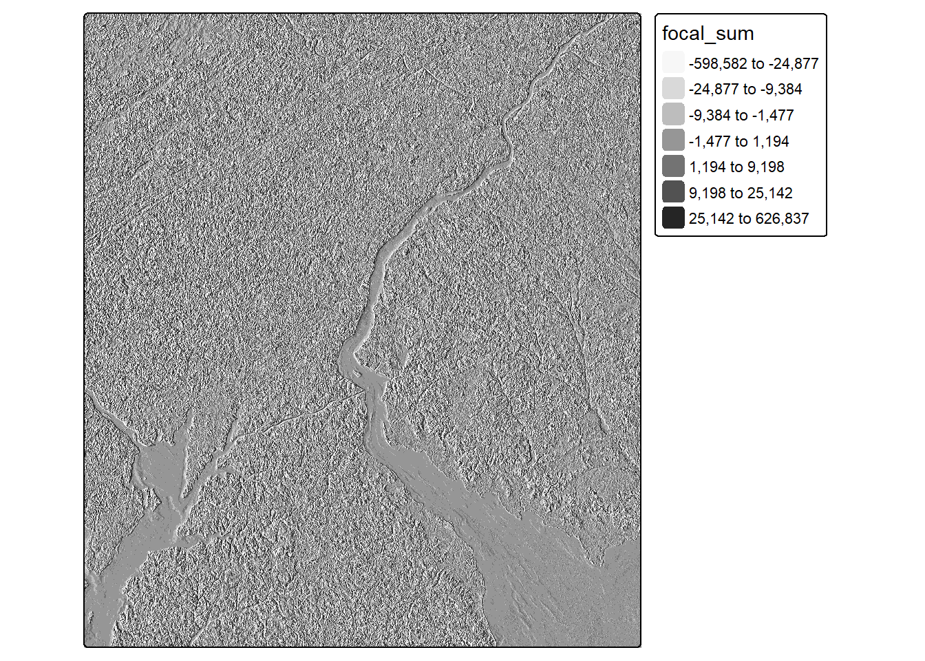
tm_shape(nir_edgey)+
      tm_raster(col.scale = tm_scale_intervals(n=7,
                                          style="quantile",
                                          values = "brewer.greys"))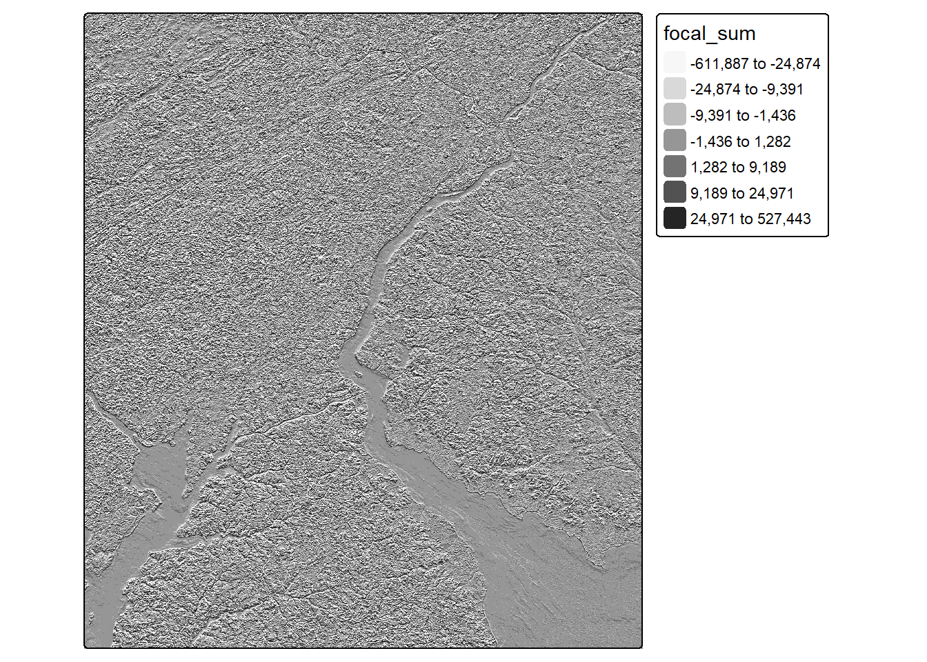
2.4 Digital Terrain Analysis
In this last section of the chapter, we explore variables that can be derived from a DTM. These surface are commonly termed digital terrain variables or land surface parameters (LSPs). For our example data, we read in a DTM provided by the USGS 3DEP. In order to speed up the computation, the DTM is degraded from a 1 m to a 5 m spatial resolution by calculating the average of the 25 cells that fall within the new larger cells.
dtm <- rast(str_glue("{folderPath}dtm.tif")) |>
  aggregate(fact=5, fun=mean)

tm_shape(dtm)+
        tm_raster(col.scale = tm_scale_continuous(values="-brewer.greys"))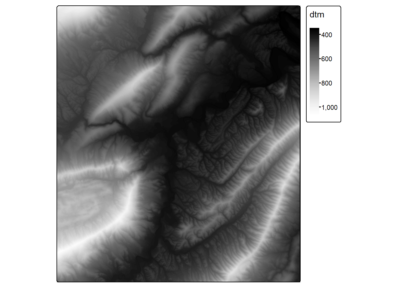
2.4.1 Common Land Surface Parameters
Table 2.2 summarizes some LSPs that can be calculated using R. The terra package can be used to calculate topographic slope and aspect while the spatialEco package adds additional functionality. If you are interested in reading more about the use of LSPs in remote sensing and spatial predictive modeling, we recommend the following papers:
Franklin, S.E., 2020. Interpretation and use of geomorphometry in remote sensing: a guide and review of integrated applications. International Journal of Remote Sensing, 41(19), pp.7700-7733.
Maxwell, A.E. and Shobe, C.M., 2022. Land-surface parameters for spatial predictive mapping and modeling. Earth-Science Reviews, 226, p.103944.
The geodl package can calculate several LSPs use fast GPU-based computation by leveraging the torch package. We will discuss this in the third section of the text.
The terra package provides the terrain() function that can calculate topographic slope, topographic aspect, the topographic position index (TPI), the topographic roughness index (TRI), and several other measures. Below, we have used this function to calculate slope and aspect in radian units. Radian units are used, as opposed to degrees, since the shade() function from terra, which is used to calculate a hillshade in the same code block, expects radian units. We specifically calculate the hillshade using a sun angle of 45-degrees and a sun azimuth or direction of 315-degrees (i.e., northwest). The hillshade is then plotted using tmap.
library(readr)
library(gt)
#| eval: true
#| echo: false
#| include: true
#| error: false
#| message: false
#| warning: false
#| results: false

dTypes <- read_csv("tables/terrainDerivatives.csv")
Rows: 13 Columns: 4
── Column specification ────────────────────────────────────────────────────────
Delimiter: ","
chr (4): Land Surface Parameter, Description, Package, Function
ℹ Use `spec()` to retrieve the full column specification for this data.
ℹ Specify the column types or set `show_col_types = FALSE` to quiet this message.dTypes |> gt() |>
fmt_markdown(columns=c(Package, Function)) |>
tab_style(
style = list(
cell_text(align="center", weight="bold")
),
locations = cells_column_labels()) |>
tab_style(
style = list(
cell_text(align="center")),
locations = cells_body(-Description)) |>
tab_caption(caption=md("**Table 2.2.** Land surface parameters (LSPs)."))| Land Surface Parameter | Description | Package | Function |
|---|---|---|---|
| Topographic Slope | Steepness | terra |
terrain() |
| Topographic Aspect | Slope orientation | terra |
terrain() |
| Hillshade | Shaded relief surface | terra |
shade() |
| Profile Curvature | Curvature in the direction of maximum slope | spatialEco |
curvature() |
| Planform Curvature | Curvature in the direction perpendicular to the direction of maximum slope | spatialEco |
curvature() |
| Total Curvature | Sigma of profile and planform curvature | spatialEco |
curvature() |
| Topographic Position Index (TPI) | (Elev - Mean); relative topographic position | spatialEco |
tpi() |
| Topographic Roughness Index (TRI) | Square root of standard deviation of slope in local window; measure of rugosity | spatialEco |
tri() |
| Topographic Dissection Index (TDI) | (Elev - Min)/(Max - Min); measure of incision | spatialEco |
dissection() |
| Surface Area Ratio (SAR) | Resolution^2 * cos( (degrees(slope) * (pi / 180); transform of steepness | spatialEco |
sar() |
| Surface Relief Ratio | (Mean - Min)/(Max - Min); measure of rugosity | spatialEco |
srr() |
| Heat Load Index (HLI) | 0 (coolest) to 1(hottest) based on aspect, slope, and latitude | spatialEco |
hli() |
| Solar-Radiation Aspect Index (TRASP) | (1 - cos((pi/180)(aspect in degrees-30) ) / 2; aspect transformation | spatialEco |
trasp() |
slp <- terrain(dtm, v ="slope", unit="radians")
asp <- terrain(dtm, v ="aspect", unit="radians")

hs <- shade(slp, asp, angle=45, direction=315)

tm_shape(hs)+
        tm_raster(col.scale = tm_scale_continuous(values="-brewer.greys"))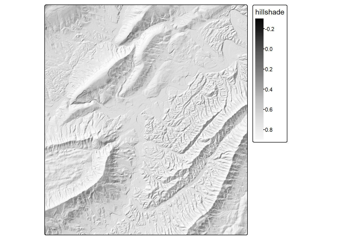
A multidirectional hillshade can be calculated by averaging hillshades created using multiple sun positions. In our example, we create hillshades using north, northwest, west, and southeast illuminations. We then average these but with double-weighting applied to the northwest illumination.
hsN <- shade(slp, asp, angle=45, direction=0)
hsNW <- shade(slp, asp, angle=45, direction=315)
hsW <- shade(slp, asp, angle=45, direction=270)
hsSE <- shade(slp, asp, angle=45, direction=135)

hsMD <- (hsN + (2*hsNW) + hsW + hsSE)/5

tm_shape(hsMD)+
        tm_raster(col.scale = tm_scale_continuous(values="-brewer.greys"))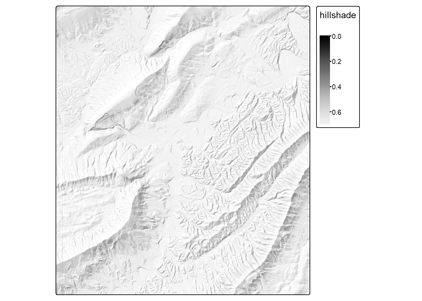
2.4.2 Other Land Surface Parameters
The spatialEco package provides additional functions for calculating land surface parameters including surface curvatures, the topographic dissection index (TDI), the heat load index (HLI), the surface area ratio (SAR), the surface relief ratio (SRR), the topographic position index (TPI), the topographic roughness index (TRI), and the topographic radiation aspect index after Roberts and Cooper (1989) (TRASP). Several of these surfaces are generated and visualized below. Some of the measures allow for defining the size of the moving window. Larger values generally yield more generalized results.
crvT <- curvature(dtm,
                  type="total")

tm_shape(crvT)+
          tm_raster(col.scale = tm_scale_intervals(n=7,
                                                   style="quantile",
                                                   values="-brewer.greys"),
                    col.legend = tm_legend(title="Total Curvature"))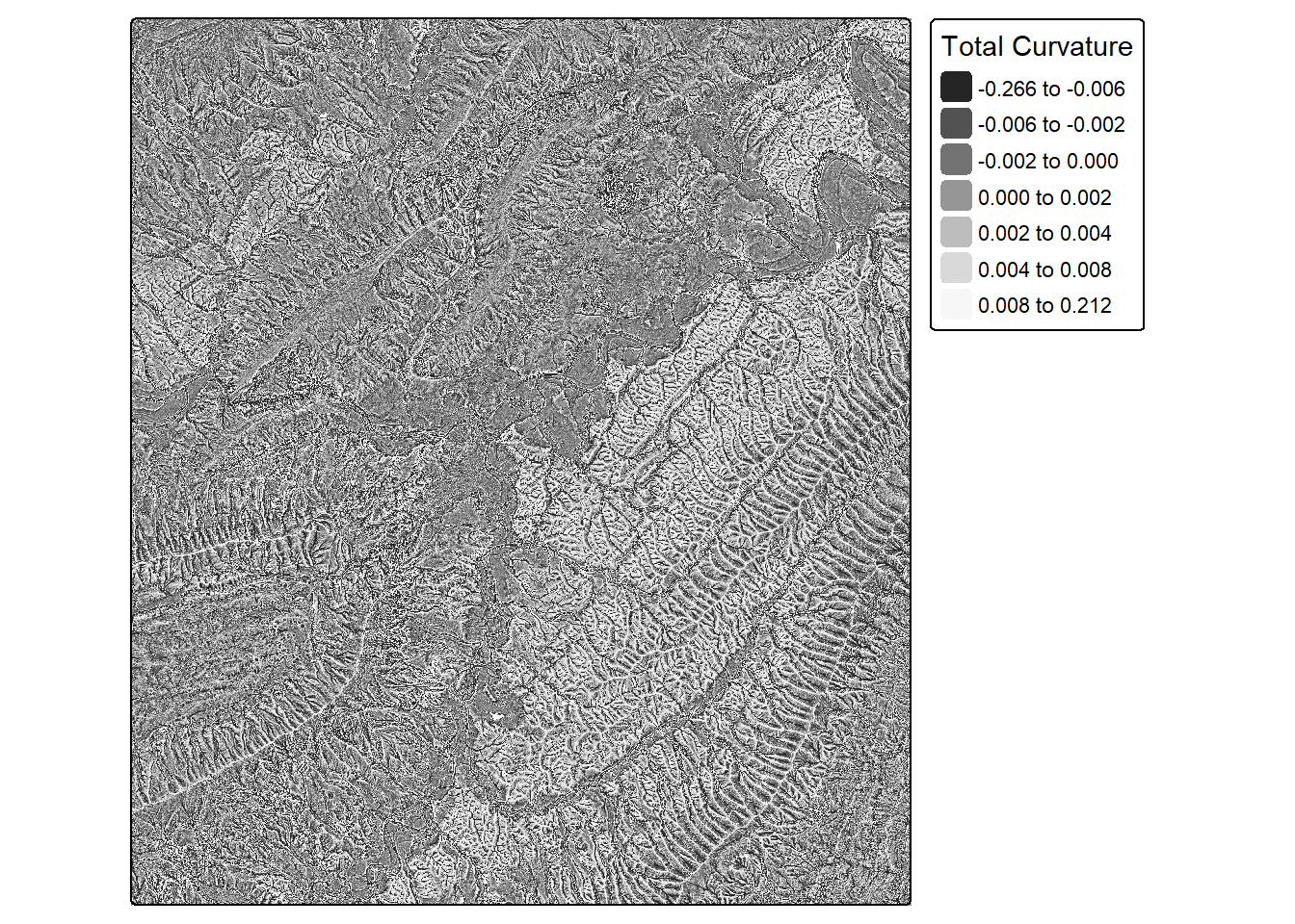
tdi <- dissection(dtm, s=7)

tm_shape(tdi)+
          tm_raster(col.scale = tm_scale_continuous(values="-brewer.greys"),
                    col.legend = tm_legend(title="TDI"))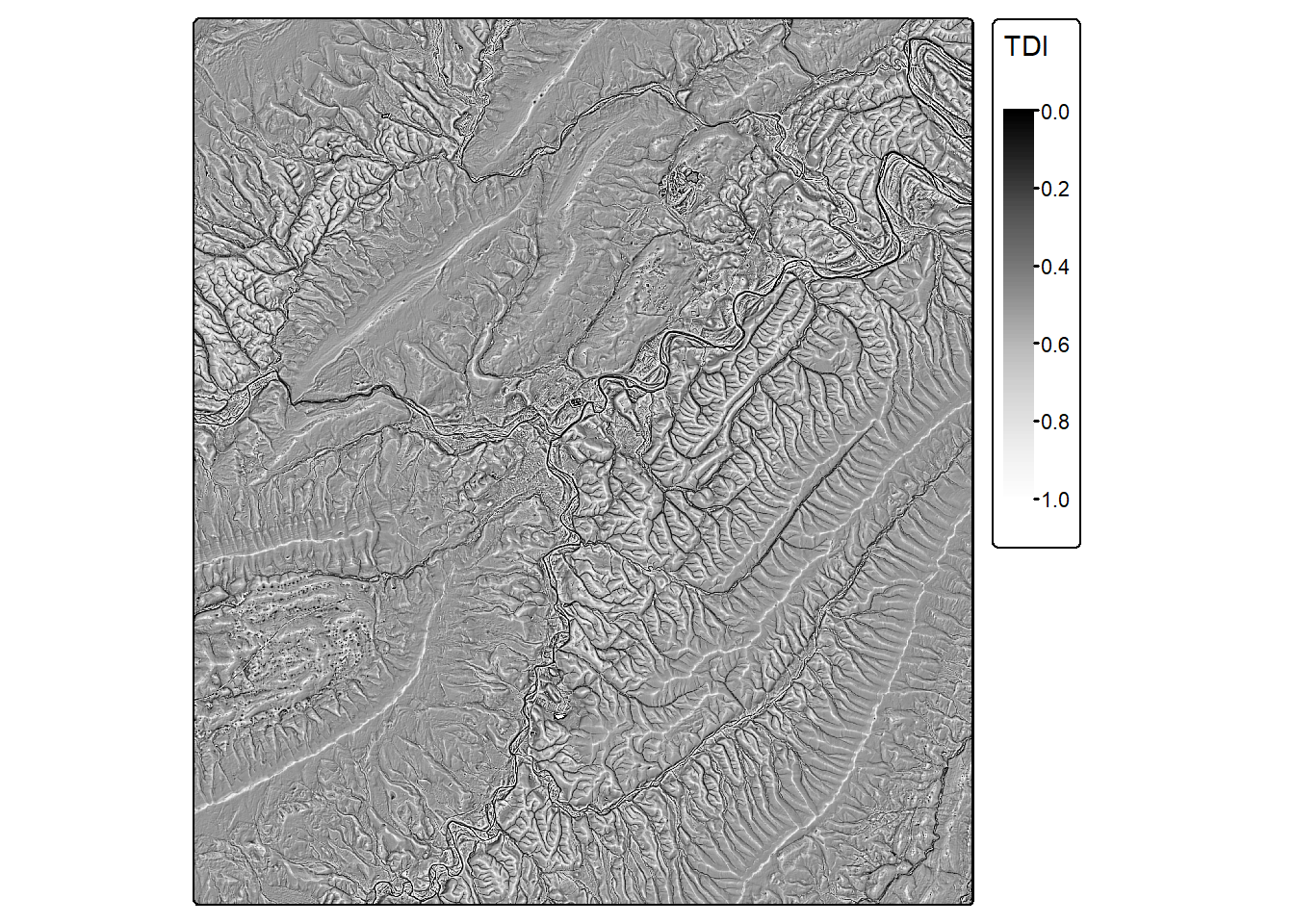
hli <- hli(dtm)

tm_shape(hli)+
          tm_raster(col.scale = tm_scale_intervals(n=7,
                                                   style="quantile",
                                                   values="-brewer.greys"),
                    col.legend = tm_legend(title="HLI"))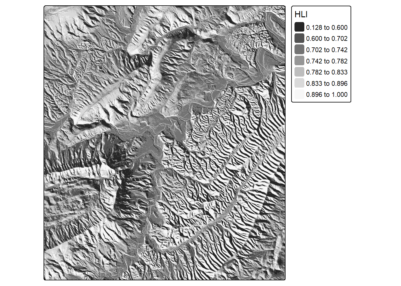
sar <- sar(dtm)
tm_shape(sar)+
        tm_raster(col.scale = tm_scale_intervals(n=7,
                                                   style="quantile",
                                                   values="-brewer.greys"),
                  col.legend = tm_legend(title="SAR"))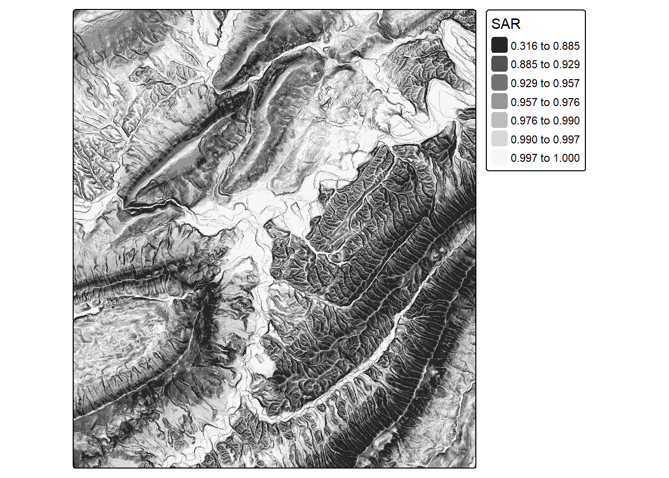
srr <- srr(dtm, s=7)
tm_shape(srr)+
        tm_raster(col.scale = tm_scale_continuous(values="-brewer.greys"),
                  col.legend = tm_legend(title="SRR"))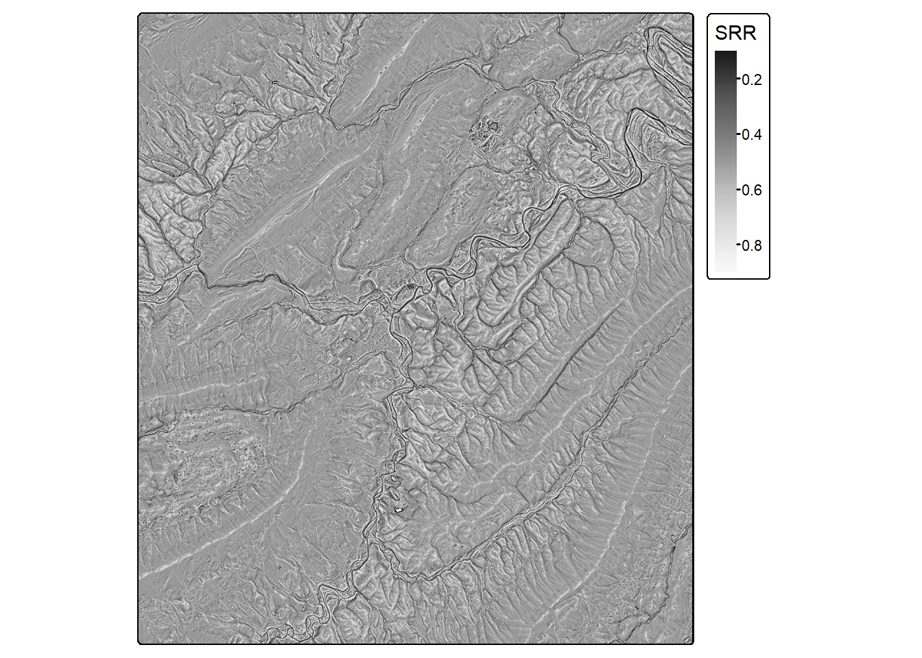
tpi <- tpi(dtm,
           scale=35,
           win="circle")

tm_shape(tpi)+
        tm_raster(col.scale = tm_scale_continuous(values="-brewer.greys"),
                  col.legend = tm_legend(title="TPI"))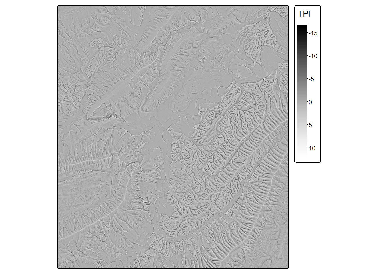
trasp <- trasp(dtm)

tm_shape(trasp)+
        tm_raster(col.scale = tm_scale_continuous(values="-brewer.greys"),
                  col.legend = tm_legend(title="TRASP"))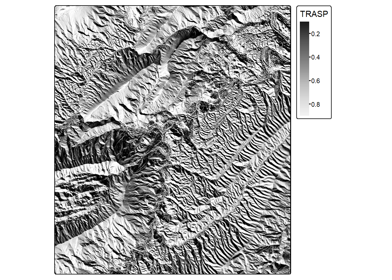
As an aside, you may be interested in removing extreme values from the generated LSPs or truncating the range of values maintained in the output. This can be accomplished using the clamp() function from terra. In the example below, we truncate the range of TPI values to be between -10 and 10.
tpi2 <- clamp(tpi, -10, 10, values=TRUE)
tm_shape(tpi2)+
        tm_raster(col.scale = tm_scale_continuous(values="-brewer.greys"),
                  col.legend = tm_legend(title="TPI"))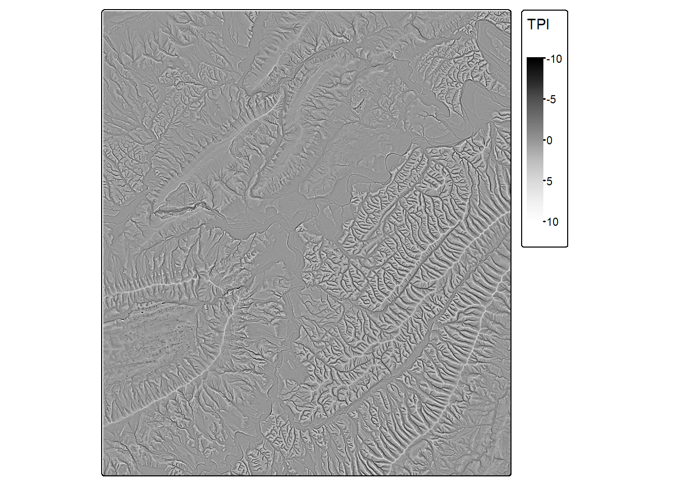
2.4.3 Customizing Moving Windows
The multiscaleDTM package allows for defining custom moving windows with varying sizes and shapes. These user-defined moving windows can be used to generate LSPs. In the final example below, we create an annulus moving window with a 10 m inner and 25 m outer radius at a 5 m spatial resolution to match the input DTM data. We then manually calculate the TPI using this custom moving window. Specifically, the mean of the cells in the moving window are subtracted from the center cell value. Next, we clamp the range from -10 to 10 and rescale the TPI to values between 0 and 1.
fAnnulus <- MultiscaleDTM::annulus_window(radius = c(10,25),
                                          unit = "map",
                                          resolution = 5)
tpiA <- dtm - terra::focal(dtm,
                           fAnnulus,
                           "mean",
                           na.rm = TRUE)

tpiA2 <- terra::clamp(tpiA,
                      -10,
                      10,
                      values = TRUE)
tpiA3 <- (tpiA2 - (-10))/(10-(-10))

tm_shape(tpiA3)+
          tm_raster(col.scale = tm_scale_continuous(values="-brewer.greys"),
                    col.legend = tm_legend(title="TPI"))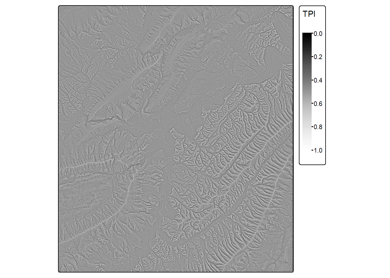
2.5 Concluding Remarks
The goal of the first two chapters of this text was to introduce you to general raster processing in R with a focus on the terra package. This is important since input predictor variables for spatial predictive modeling tasks are commonly represented as raster grids. Further, we find that we spend a lot of time obtaining and preprocessing raster data. In other words, this is an important skill set for geospatial scientists and modelers. The next chapter wraps up our discussion of preprocessing with a more general discussion of feature engineering using the parsnips package.
2.6 Questions
- Based on the spectral reflectance properties of vegetation, explain why the normalized difference vegetation index (NDVI) is valuable for assessing for the presence of vegetation and vegetation health.
- Based on the spectral reflectance properties of snow, explain why the normalized difference snow index (NDSI) is valuable for assessing for the presence of snow.
- When performing a principal component analysis (PCA), explain the difference between eigenvalues and eigenvectors.
- Explain why principal component analysis is a linear transformation of the original variables.
- Explain the difference between profile and planform curvature.
- Explain how topographic slope is calculated from a digital terrain model (DTM) using a 3x3 cell moving window.
- Topographic aspect in radian units can be converted to a measure of “northwardness” as the cosine of the aspect while it can be converted to a measure of “eastwardness” as the sine of the aspect. Mathematically, explain why using sine and cosine transformations can accomplish these desired transformations.
- Explain the equation used to calculate a hillshade from a slope and aspect surfaces.
2.7 Exercises
You have been provided with the following files in the exercise folder for the chapter. All raster grids/images have a 10 m spatial resolution. All layers are projected into WGS84 UTM Zone 18N.
- loff.tif: Sentinel-2 Multispectral Instrument (MSI) leaf-off image for portion of central Pennsylvania
- lon.tif: Sentinel-2 Multispectral Instrument (MSI) leaf-on image for portion of central Pennsylvania
- dtm2.tif: digital terrain model (DTM) with elevation in meters
- chpt2.gpkg/extent2: study area extent in central Pennsylvania
- chpt2.gpkg/pnts2: plot locations
Complete the following tasks:
- Read in all of the files
- Use tmap to display the extent and point features
- Rename the leaf-off image bands as follows: “offBlue”, “offGreen”, “offRed”, “offNIR”, “offSWIR1”, “offSWIR2”
- Rename the leaf-on image bands as follows: “onBlue”, “onGreen”, “onRed”, “onNIR”, “onSWIR1”, “onSWIR2”
- Visualize the two images using terra as false color composites
- Use tmap to visualize the DTM data
- Align the two images to the DTM data using cubic convolution
- Calculate the normalized difference vegetation index (NDVI) separately for both images
- From the DTM, calculate topographic slope
- Stack the leaf-off image bands, leaf-on image bands, leaf-off NDVI, leaf-on NDVI, elevation, and slope into a single object
- Make sure all bands have meaningful names
- Extract all the band values at the point locations
- Save a copy of the point layer to disk with all the raster layer values include in the attribute table