10 Tensors
10.1 Topics Covered
- Understand torch tensors and the need for this new data model
- Obtain and understand tensor data characteristics
- Understand and define torch data types
- Move tensors between the CPU and GPU
- Convert base R data types to tensors
- Convert tabulated data to tensors
- Convert raster grids to torch tensors
- Reshape tensors
- Perform math and logical operations on tensors
- Aggregate and summarize tensors
- Subset tensors using bracket notation
10.2 Introduction
This section of the text focuses on deep learning. There are multiple packages or environments available in R for implementing deep learning including Tensforflow/Keras and torch. We focus on torch and associated packages. torch allows for implementing deep learning in R without the need to interface with a Python/PyTorch environment. It makes use of the C++ libtorch library and supports graphics processing unit (GPU) acceleration. We use the luz package to simplify the training process and geodl to implement geospatial semantic segmentation.
Before exploring deep learning methods, we need to describe the tensor data model used with deep learning. In the context of deep learning, tensors are multidimensional arrays, similar to an R vector, matrix, or array. Given the need to be able to use GPU- and CPU-based computation, it is necessary to use a data model that allows for moving data between devices. In order to implement backpropagation, it is necessary to keep track of the mathematical operations performed on tensors. This supports the calculation of the gradient of the loss with respect to model parameters, which is required to update these parameters and allow the algorithm to “learn”. Tensors support these operations; thus, it is important to understand the tensor data model and how it is specifically implemented with torch in order to implement deep learning in this environment.
If you want to follow along with this section of the text, you will need to install the torch package. Since we will be working with complex models and geospatial data, you will also need to set up GPU-based computation. Directions for setting up torch with GPU support can be found [here]. You also need a graphics card that supports deep learning computation and to set up NVIDIA’s Compute Unified Device Architecture (CUDA) with the correct version. CUDA is free.
10.3 Tensor Data
10.3.1 Tensor from R Array
It is possible to create torch tensors from base R data types. In our first example, we generate an R vector of all odd integer values between 1 and 150. These data are then converted to an R array using the array() function. The array has a shape of [5,5,3]; as a result, 75 values are needed to fill it. To convert the array to a torch tensor, we use the torch_tensor() function. Once a torch tensor is created, its data type can be obtained using the dtype property. Its shape, or the length of each dimension, can be obtained with shape while the device on which it is stored can be obtained using device. the t1 tensor has a torch_float data type, a shape of [5,5,3], and is currently housed on the CPU.
The torch-based code that we will use in this section of the text looks a bit different from more typical R code since it makes use of classes and subclassing.
data2 <- seq(from=1,
             to=150,
             by=2)
rnames <- c("R1",
            "R2",
            "R3",
            "R4",
            "R5")
cnames <- c("C1",
            "C2",
            "C3",
            "C4",
            "C5")
bnames <- c("B1",
            "B2",
            "B3")
array1 <- array(data2, c(5, 5, 3),
                dimnames=list(rnames,
                              cnames,
                              bnames))
print(array1)
, , B1
C1 C2 C3 C4 C5
R1 1 11 21 31 41
R2 3 13 23 33 43
R3 5 15 25 35 45
R4 7 17 27 37 47
R5 9 19 29 39 49
, , B2
C1 C2 C3 C4 C5
R1 51 61 71 81 91
R2 53 63 73 83 93
R3 55 65 75 85 95
R4 57 67 77 87 97
R5 59 69 79 89 99
, , B3
C1 C2 C3 C4 C5
R1 101 111 121 131 141
R2 103 113 123 133 143
R3 105 115 125 135 145
R4 107 117 127 137 147
R5 109 119 129 139 149t1 <- torch_tensor(array1)
t1$dtypetorch_Floatt1$shape[1] 5 5 3t1$devicetorch_device(type='cpu')The code below shows how to move a tensor to the GPU using the to() method for torch tensors. device="cuda" indicates to move the data to an available CUDA-enabled GPU. The data can be moved back to the CPU using to(device="cpu"). If you get an error when trying to move the tensor, there may be an issue with your CUDA installation.
t2 <- t1$to(device="cuda")
t2$device
torch_device(type='cuda', index=0)10.3.2 Tensor Creation Functions
There are several built-in torch functions for generating tensors including:
-
torch_zeros(): create tensor of a defined shape filled with zeros -
torch_ones(): create tensor of a defined shape filled with ones -
torch_rand(): generate floating point values from a uniform distribution between zero and one -
torch_randn(): generate floating point values from a normal distribution with a mean of zero and a standard deviation of one
In the examples below, the provided numbers indicate the desired shape of the output. For example, in the torch_zeros() example, a tensor with a shape of [3,5] is created, which contains 3 rows and 5 columns of zero values. By default, all of these functions generate data with a float data type stored on the CPU. This is indicated by CPUFloatType.
tZeros <- torch_zeros(3,5)
tZeros
torch_tensor
0 0 0 0 0
0 0 0 0 0
0 0 0 0 0
[ CPUFloatType{3,5} ]tOnes <- torch_ones(4,4)
tOnestorch_tensor
1 1 1 1
1 1 1 1
1 1 1 1
1 1 1 1
[ CPUFloatType{4,4} ]tRnd <- torch_rand(3,5)
tRndtorch_tensor
0.5559 0.5905 0.8285 0.1799 0.2547
0.6825 0.3606 0.7551 0.1546 0.3739
0.7069 0.8996 0.9565 0.8288 0.6619
[ CPUFloatType{3,5} ]tRndN <- torch_randn(3,5)
tRndNtorch_tensor
0.9826 -0.0474 -1.8642 -0.5371 -0.1695
0.4395 0.7970 -1.2473 0.3499 1.3742
1.3869 -1.1803 0.2269 1.0906 0.8362
[ CPUFloatType{3,5} ]10.3.3 Tensor Characteristics
A variety of properties are available to obtain information about tensors:
-
dtype: data type -
device: device storing data -
shape: shape of tensor -
ndim: number of dimensions
The first example demonstrates a means to create a tensor of integer values using torch_randint(). Random values between 0 and 255 are selected to fill a tensor with a shape of [3,128,128]. This is meant to mimic a 3-band, 8-bit image with 128 rows and 128 columns of pixels.
tRndI <- torch_randint(low=0,
                       high=255,
                       c(3, 128, 128))
tRndI$dtypetorch_FloattRndI$devicetorch_device(type='cpu')tRndI$shape[1] 3 128 128tRndI$ndim[1] 3Within torch_tensor(), the dtype argument is used to explicitly define the desired data type. Available data types include the following. We most commonly use torch_float32() and torch_int64() for deep learning tasks. There are also data types for complex numbers, which are not listed or discussed here.
-
torch_float32(): floating point -
torch_float64(): double -
torch_float16(): half precision float -
torch_unint8(): unsigned 8-bit integer -
torch_int8(): signed 8-bit integer -
torch_int16(): signed 16-bit integer -
torch_int32(): signed 32-bit integer -
torch_int64(): signed 64-bit integer -
torch_bool(): Boolean/logical, TRUE or FALSE, or 0/1
In the first example below, we explicitly set the data type to torch_int64(), or a long integer. We also use the device argument to place the tensor on the GPU. This is an alternative to using the device() method. In the second example, we use the torch_float32() data type.
rndInts <- sample(0:255,
                  20,
                  replace = TRUE)
t1 <- torch_tensor(rndInts,
                   dtype=torch_int64(),
                   device="cuda")
t1$dtypetorch_Longt1$devicetorch_device(type='cuda', index=0)t1$shape[1] 20t1$ndim[1] 1imgT <- sample(0:255,
300,
replace=TRUE) |>
array(dim = c(3,10,10)) |>
torch_tensor(dtype=torch_float32(),
device="cuda")
imgT$dtypetorch_FloatimgT$devicetorch_device(type='cuda', index=0)imgT$shape[1] 3 10 10imgT$ndim[1] 310.3.4 Tensor from Tabulated Data
Tensors can also be generated from data files. The code block below demonstrates how to convert a CSV file, read into R as a tibble, into a tensor. First, the data are read using read_csv() from readr with some additional manipulation using dplyr. Next, columns that represent predictor variables are normalized using recipes from tidymodels. This requires defining a recipe (recipe()), preparing the recipe (prep()), and using it to augment the data (bake()). The dependent variable (“class”) is then dropped from the table, the remaining columns are converted to an R matrix, and the matrix is converted to a torch tensor with a torch_float32() data type. As a check, ndim confirms that the tensor has two dimensions while shape confirms that it has a shape of [16558, 10]: there are 16,558 observations and 10 variables.
fldPth <- "gslrData/chpt10/data/"

euroSatTrain <- read_csv(str_glue("{fldPth}train_aggregated.csv")) |>
  mutate_if(is.character,
            as.factor) |>
  select(-1, -code)

myRecipe <- recipe(class ~ .,
                   data = euroSatTrain) |>
  step_normalize(all_numeric_predictors())

myRecipePrep <- prep(myRecipe,
                     training=euroSatTrain)

trainProcessed <- bake(myRecipePrep,
                       new_data=NULL)

trainT <- trainProcessed |>
  select(-class) |>
  as.matrix() |>
  torch_tensor(dtype=torch_float32(),
               device="cuda")

trainT$ndim
[1] 2trainT$shape[1] 16558 1010.3.5 Tensor from Raster Data
Other types of data can be converted to torch tensors other than tabulated data. This next example demonstrates how to convert a multiband raster grid, a Landsat 8 Operational Land Imager (OLI) multispectral image, to a torch tensor. The data are first read in as a spatRaster object using terra, which is then converted to an R array followed by a torch tensor. We explicitly set the data type to torch_float32() and move the data to the GPU. The shape of the tensor is [4007,3521,7]: rows, columns, bands. In the following code block, we convert the torch tensor back to a spatRaster object. The detach() method is used to stop keeping track of the operations performed on the tensor (i.e., detach it from the computational graph) while to() is used to move the data to the CPU. Once on the CPU, the data are converted to an R array followed by a spatRaster object. Since the spatial reference information was not maintained when the raster was converted to a tensor, it is necessary to specify the extent and coordinate reference system using the original spatRaster object.
folderPath <- "gslrData/chpt10/data/"

lOff <- rast(str_glue("{folderPath}ls8_3_11_2024_SR.tif"))

names(lOff) <- c("Edge",
                 "Blue",
                 "Green",
                 "Red",
                 "NIR",
                 "SWIR1",
                 "SWIR2")

plotRGB(lOff,
        r=7,
        g=5,
        b=3,
        stretch="lin")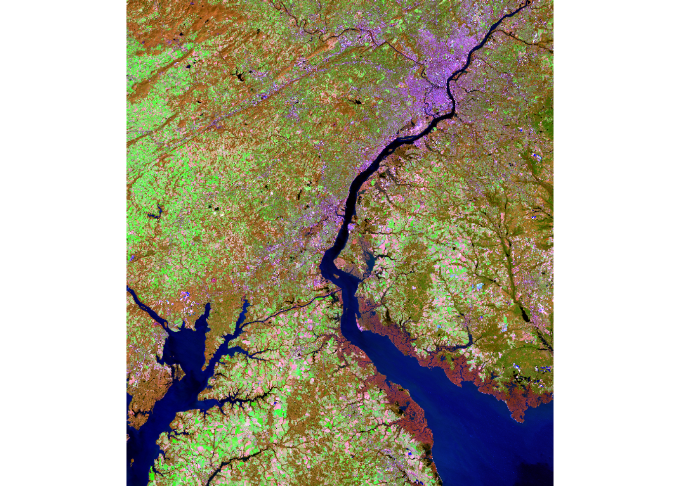
lOffT <- lOff|>
  as.array() |>
  torch_tensor(dtype=torch_float32(),
               device="cuda")

lOffT$shape
[1] 4007 3521 7
10.4 Reshape Tensors
10.4.1 Permute
We now explore a variety of operations that can be performed on tensor data. The permute() method is used to change the order of the dimensions in the tensor. In the raster example above, we may need to represent the data using the order bands, rows, columns as opposed to rows, columns, bands. Permute can accomplish this task. This is demonstrated in the code block for a new tensor where the last dimension is moved to the first position. The new order is defined using a vector of dimension indices.
torch and torchvision use a channels-first as opposed to channels-last configuration while terra uses channels-last. Permute can be used to change the order as needed.
imgT <- torch_randint(low=0,
                      high=255,
                      c(128, 128, 3))
imgT2 <- imgT$permute(c(3,1,2))
imgT2$shape
[1] 3 128 12810.4.2 Squeeze and Unsqueeze
unsqueeze() is used to add a dimension with a length of one. For example, a grayscale image could be represented at [Channels, Width, Height] or [Width, Height]. In other words, since there is only one band there is no need to differentiate bands using a third dimension. However, some operations may expect the channel dimension to be included, even if it has a length of one. In our first example, we generate a tensor without a channel dimension then add the channel dimension at position 1 using dim=1. We could add this dimension at the end using dim=3.
In contrast to unsqueeze(), squeeze() removes dimensions with a length of one as demonstrated in the second example.
imgT <- torch_randint(low=0,
                      high=255,
                      c(128, 128))
imgT$shape
[1] 128 128imgT <- imgT$unsqueeze(dim=1)
imgT$shape[1] 1 128 128imgT <- imgT$squeeze()
imgT$shape[1] 128 12810.4.3 View
view() is used to represent the data using a new shape or number of dimensions. Generally, the number of values must fill the new shape exactly. In the first example, we collapse a tensor with a shape of [128,128] to a single dimension with a length of [16384]. If the required length of one dimensions is not known, -1 can be used in its associated position, and torch will determine the required length as long as a length can be selected that allows for the set of values to perfectly fill the tensor.
imgTFlat <- imgT$view(128*128)
imgTFlat$shape
[1] 16384imgTFlat <- imgT$view(c(64,-1))
imgTFlat$shape[1] 64 25610.5 Tensor Math and Logic
10.5.1 Operations on Tensors
We now explore performing mathematical and logical operations on tensors. We start by creating two tensors of random values each with a shape of [5,5].
t1 <- torch_rand(5,5)
t2 <- torch_rand(5,5)

t1
torch_tensor
0.0773 0.4172 0.6537 0.4066 0.1142
0.7344 0.0837 0.3125 0.0369 0.9699
0.7415 0.5849 0.3394 0.8616 0.5022
0.1624 0.2891 0.6697 0.9948 0.0144
0.5658 0.4757 0.9706 0.0282 0.4456
[ CPUFloatType{5,5} ]t2torch_tensor
0.3730 0.3651 0.7658 0.6224 0.7958
0.8948 0.2385 0.9572 0.9916 0.4030
0.7425 0.4394 0.9028 0.5198 0.2516
0.4769 0.4893 0.7827 0.8176 0.1448
0.7991 0.7806 0.9405 0.6656 0.1545
[ CPUFloatType{5,5} ]Basic math and logical operations are demonstrated in the next code blocks including greater than, addition, subtraction, multiplication, division, and exponentiation. The syntax is identical to that used in base R for vectors, arrays, and matrices; however, the returned object will be a tensor. Note that logical tests return a tensor of 0/1 values with a torch_bool() data type where 0 indicates FALSE and 1 indicates TRUE. All other operations return a torch_float32() data type, the same as the input tensor. It is also possible to perform operations between two tensors as long as they have the same shape or meet required broadcasting rules. We will not discuss broadcasting here.
#greater than
t1 > .3
torch_tensor
0 1 1 1 0
1 0 1 0 1
1 1 1 1 1
0 0 1 1 0
1 1 1 0 1
[ CPUBoolType{5,5} ]#addition
t1+1torch_tensor
1.0773 1.4172 1.6537 1.4066 1.1142
1.7344 1.0837 1.3125 1.0369 1.9699
1.7415 1.5849 1.3394 1.8616 1.5022
1.1624 1.2891 1.6697 1.9948 1.0144
1.5658 1.4757 1.9706 1.0282 1.4456
[ CPUFloatType{5,5} ]#subtraction
t1-.5torch_tensor
-0.4227 -0.0828 0.1537 -0.0934 -0.3858
0.2344 -0.4163 -0.1875 -0.4631 0.4699
0.2415 0.0849 -0.1606 0.3616 0.0022
-0.3376 -0.2109 0.1697 0.4948 -0.4856
0.0658 -0.0243 0.4706 -0.4718 -0.0544
[ CPUFloatType{5,5} ]#multiplication
t1*2torch_tensor
0.1546 0.8345 1.3074 0.8132 0.2283
1.4688 0.1673 0.6251 0.0738 1.9398
1.4830 1.1698 0.6787 1.7232 1.0044
0.3247 0.5782 1.3393 1.9897 0.0289
1.1316 0.9514 1.9412 0.0564 0.8912
[ CPUFloatType{5,5} ]#division
t1/2torch_tensor
0.0387 0.2086 0.3268 0.2033 0.0571
0.3672 0.0418 0.1563 0.0184 0.4849
0.3708 0.2924 0.1697 0.4308 0.2511
0.0812 0.1445 0.3348 0.4974 0.0072
0.2829 0.2378 0.4853 0.0141 0.2228
[ CPUFloatType{5,5} ]#exponentiation
t1**3torch_tensor
4.6206e-04 7.2637e-02 2.7932e-01 6.7227e-02 1.4876e-03
3.9606e-01 5.8538e-04 3.0528e-02 5.0163e-05 9.1238e-01
4.0771e-01 2.0009e-01 3.9083e-02 6.3958e-01 1.2666e-01
4.2794e-03 2.4157e-02 3.0032e-01 9.8460e-01 3.0105e-06
1.8114e-01 1.0764e-01 9.1443e-01 2.2425e-05 8.8463e-02
[ CPUFloatType{5,5} ]#greater than
t1>t2torch_tensor
0 1 0 0 0
0 0 0 0 1
0 1 0 1 1
0 0 0 1 0
0 0 1 0 1
[ CPUBoolType{5,5} ]#addition
t1+t2torch_tensor
0.4503 0.7823 1.4195 1.0290 0.9100
1.6291 0.3221 1.2697 1.0285 1.3729
1.4841 1.0243 1.2422 1.3814 0.7538
0.6393 0.7784 1.4524 1.8124 0.1592
1.3649 1.2563 1.9111 0.6938 0.6001
[ CPUFloatType{5,5} ]#subtraction
t1-t2torch_tensor
-0.2956 0.0522 -0.1122 -0.2158 -0.6817
-0.1604 -0.1548 -0.6446 -0.9547 0.5669
-0.0010 0.1454 -0.5635 0.3417 0.2506
-0.3146 -0.2002 -0.1130 0.1773 -0.1303
-0.2333 -0.3049 0.0301 -0.6374 0.2910
[ CPUFloatType{5,5} ]#multiplication
t1*t2torch_tensor
0.0288 0.1523 0.5006 0.2531 0.0908
0.6571 0.0199 0.2992 0.0366 0.3909
0.5506 0.2570 0.3064 0.4479 0.1264
0.0774 0.1414 0.5242 0.8133 0.0021
0.4521 0.3713 0.9129 0.0188 0.0689
[ CPUFloatType{5,5} ]#division
t1/t2torch_tensor
0.2073 1.1429 0.8536 0.6533 0.1434
0.8208 0.3508 0.3265 0.0372 2.4065
0.9986 1.3310 0.3759 1.6574 1.9956
0.3404 0.5908 0.8556 1.2168 0.0997
0.7081 0.6094 1.0320 0.0424 2.8833
[ CPUFloatType{5,5} ]#exponentiation
t1**t2torch_tensor
0.3849 0.7268 0.7221 0.5712 0.1778
0.7586 0.5534 0.3285 0.0379 0.9878
0.8009 0.7900 0.3769 0.9255 0.8409
0.4202 0.5449 0.7306 0.9958 0.5414
0.6344 0.5599 0.9723 0.0930 0.8826
[ CPUFloatType{5,5} ]There are methods and functions available to implement many math and logic operations. The first three examples below demonstrate methods while the last two demonstrate functions.
t1$add(t2)torch_tensor
0.4503 0.7823 1.4195 1.0290 0.9100
1.6291 0.3221 1.2697 1.0285 1.3729
1.4841 1.0243 1.2422 1.3814 0.7538
0.6393 0.7784 1.4524 1.8124 0.1592
1.3649 1.2563 1.9111 0.6938 0.6001
[ CPUFloatType{5,5} ]t1$subtract(t2)torch_tensor
-0.2956 0.0522 -0.1122 -0.2158 -0.6817
-0.1604 -0.1548 -0.6446 -0.9547 0.5669
-0.0010 0.1454 -0.5635 0.3417 0.2506
-0.3146 -0.2002 -0.1130 0.1773 -0.1303
-0.2333 -0.3049 0.0301 -0.6374 0.2910
[ CPUFloatType{5,5} ]t1$multiply(t2)torch_tensor
0.0288 0.1523 0.5006 0.2531 0.0908
0.6571 0.0199 0.2992 0.0366 0.3909
0.5506 0.2570 0.3064 0.4479 0.1264
0.0774 0.1414 0.5242 0.8133 0.0021
0.4521 0.3713 0.9129 0.0188 0.0689
[ CPUFloatType{5,5} ]torch_sin(t1)torch_tensor
0.0772 0.4052 0.6081 0.3955 0.1139
0.6701 0.0836 0.3075 0.0369 0.8248
0.6754 0.5521 0.3329 0.7589 0.4814
0.1616 0.2851 0.6207 0.8387 0.0144
0.5361 0.4580 0.8252 0.0282 0.4310
[ CPUFloatType{5,5} ]torch_sqrt(t2)torch_tensor
0.6107 0.6042 0.8751 0.7889 0.8921
0.9459 0.4883 0.9784 0.9958 0.6348
0.8617 0.6629 0.9502 0.7210 0.5016
0.6906 0.6995 0.8847 0.9042 0.3805
0.8939 0.8835 0.9698 0.8158 0.3931
[ CPUFloatType{5,5} ]10.5.2 Tensor Aggregation and Summarization
Data can be aggregated or summarized using summary metrics. The code block below demonstrates methods for calculating the mean and standard deviation. If no dim argument is specified, a single aggregated metric is returned. If you want to aggregate over certain dimensions, you can specify the dim argument. We are using c(2,3) so that a separate summary metric is returned for each channel. In other words, we are aggregating the values for just the width and height dimensions but not the channels in order to return channel-wise summary statistics.
imgT <- torch_randint(low=0,
                      high=255,
                      c(3, 128, 128))

imgT$mean()
torch_tensor
127.67
[ CPUFloatType{} ]imgT$mean(dim=c(2,3))torch_tensor
127.8914
127.2388
127.8809
[ CPUFloatType{3} ]imgT$std(dim=c(2,3))torch_tensor
73.8997
73.8067
74.0903
[ CPUFloatType{3} ]The torch_argmax() function returns the index for the largest value relative to a specific dimension. In the example, we are creating a tensor with a shape of [5, 10, 10]. As you will see in later sections, this could represent the predicted logits for five classes for each cell in a 10-by-10 window. To convert from the class logits to the predicted class label, torch_argmax() is applied since the index with the largest logit represents the numeric code for the class with the highest predicted logit.
clsL <- torch_rand(c(5, 10, 10))
clsI <- torch_argmax(clsL,
                     dim=c(1))
clsI
torch_tensor
2 5 2 5 5 5 4 3 5 2
5 4 2 2 1 4 3 4 1 1
3 2 4 1 5 5 3 4 1 1
2 4 4 1 1 5 3 1 1 4
1 1 3 5 1 5 3 4 2 1
3 4 3 3 4 5 2 2 2 5
5 3 1 5 1 3 4 5 3 4
4 3 1 5 1 2 1 3 3 3
1 5 5 4 4 4 2 5 1 1
5 3 3 4 4 1 3 2 5 5
[ CPULongType{10,10} ]10.6 Tensor Subsetting
In this last section, we discuss subsetting values from a tensor using bracket notation. This works very similar to data subsetting for base R vectors, matrices, and arrays. We begin by creating a tensor of random integer values between 0 and 255 with a shape of [3, 128, 128] to represent a 3-band, 8-bit raster image.
imgT <- torch_randint(low=0,
                      high=255,
                      c(3, 128, 128))
In the first example, we are extracting the values in band 1, rows 10 through 20, and columns 10 through 20. In the second example, we are extracting all the bands, as indicated by an empty index, and rows 4 through 8 and columns 4 through 8. The third example is the same as the second except that we now extract values from only band 1 and 2. If a non-contiguous set of indices need to be extracted, you must use c(), as demonstrated in the last example.
imgT[1, 10:20, 10:20]torch_tensor
242 127 137 7 159 66 230 217 165 85 179
117 184 146 71 6 65 49 201 165 96 168
254 201 143 147 79 163 135 142 182 183 112
229 149 50 153 3 128 106 129 92 221 99
127 235 78 97 89 159 136 220 175 74 121
171 68 12 177 95 124 231 47 149 0 138
111 159 207 62 181 90 146 179 153 64 230
132 122 84 65 116 25 150 156 189 46 219
183 78 31 146 48 69 227 36 74 244 14
136 67 192 162 82 155 89 213 150 160 131
7 124 230 7 74 219 218 65 35 117 125
[ CPUFloatType{11,11} ]imgT[,4:8,4:8]torch_tensor
(1,.,.) =
194 9 227 227 1
133 70 192 39 209
132 135 55 102 195
56 14 6 118 66
120 232 160 109 33
(2,.,.) =
182 236 36 194 10
63 118 106 96 244
96 64 36 23 241
142 73 246 132 172
253 176 169 145 238
(3,.,.) =
207 212 106 227 66
23 133 183 227 126
241 60 232 153 116
49 10 51 18 155
225 145 160 102 121
[ CPUFloatType{3,5,5} ]imgT[1:2, 4:8, 4:8]torch_tensor
(1,.,.) =
194 9 227 227 1
133 70 192 39 209
132 135 55 102 195
56 14 6 118 66
120 232 160 109 33
(2,.,.) =
182 236 36 194 10
63 118 106 96 244
96 64 36 23 241
142 73 246 132 172
253 176 169 145 238
[ CPUFloatType{2,5,5} ]imgT[c(1,3),4:8,4:8]torch_tensor
(1,.,.) =
194 9 227 227 1
133 70 192 39 209
132 135 55 102 195
56 14 6 118 66
120 232 160 109 33
(2,.,.) =
207 212 106 227 66
23 133 183 227 126
241 60 232 153 116
49 10 51 18 155
225 145 160 102 121
[ CPUFloatType{2,5,5} ]The default behavior is to drop dimensions with a length of one after subsetting, as demonstrated in the first code block. However, you can maintain dimensions with a length of one using drop=FALSE.
imgT2 <- imgT[1,4:8,4:8]
imgT2$shape
[1] 5 5imgT2 <- imgT[1,4:8,4:8, drop=FALSE]
imgT2$shape[1] 1 5 510.7 Concluding Remarks
Now that you have a basic understanding of the torch tensor data model, we can move on to using this data model to represent data for implementing deep learning. In the next chapter, we build and train a basic artificial neural network (ANN). In the following chapter, we build and train convolutional neural networks (CNN). You will also learn how to build datasets and dataloaders for representing a variety of input data as input to deep learning workflows and delivering them as mini-batches for use during the training and validation processes.
10.8 Questions
- What is the purpose of the
torch_clamp()function? - What is the difference between the
torch_argmax()andtorch_amax()functions? - What is the purpose of the
torch_dot()function? - What is the purpose of the
torch_eye()function? - Explain the difference between
tensor$shapeandtensor$ndim. - Explain the purpose of
torch_bucketize(). - How many different values can be differentiated when using the
torch_int8()data type? - Explain the difference between the
torch_half(),torch_double(), andtorch_float()data types.