6 Linear Regression
6.1 Topics Covered
- Fit a linear model
- Include higher order terms (polynomial regression)
- Fit a multiple linear regression model
- Incorporate interactions
- Interpret linear regression coefficients and summary information
- Diagnostics for regression assumptions
- L1 and L2 regularization
- Apply a linear model to raster data
6.2 Introduction
A great place to begin study supervised learning algorithms is linear regression since the process used to implement it is very similar to more advanced algorithms. Labeled samples are still necessary to train the model, and models are built using one (i.e. single or simple linear regression) or multiple (i.e., multiple linear regression) predictor variables. Outside of generating models for making predictions to new data, which is the focus of this text, linear regression is also a key component of statistical analysis. Many inferential methods, for example analysis of variance (ANOVA) make use of linear models. However, to trust the results of statistical tests that rely on linear regression, certain assumptions must be met, which are discuss and tested later in this chapter.
The linear regression model takes the following form:
\[ \begin{aligned} y &= \beta_0 + \beta_1 x + \varepsilon \\ \text{where:} \\ y &\text{ = dependent variable} \\ x &\text{ = predictor variable } \\ \beta_0 &\text{ = } \mathit{y} \text{-intercept term} \\ \beta_1 &\text{ = slope or coefficient for variable } \mathit{x} \\ \varepsilon &\text{ = error term (residual)} \end{aligned} \]
The goal of training or fitting a linear regression model is to estimate the trainable parameters or beta terms that minimizes some measure. When fitting a model using ordinary least squares (OLS) the goal is to minimize the sum of the squared residuals. A residual is the difference between the actual value and the predicted value for a sample.
Since linear models are so commonly used and important in data science and statistical inference, they can be built using base R functions, specifically the lm() function. However, packages add functionality for building, evaluating, and exploring linear models. We specifically make use of the car, lmtest, gvlma, corrplot, and glmnet packages in this chapter. Linear models can also be used to make predictions to spatial data. To work with spatial data in this chapter, we use tmap, tmaptools, and terra. Assessment metrics are implemented with yardstick while data wrangling relies on the tidyverse and reshape2.
We specifically explore the prediction of the composite burn index (CBI) using the differenced normalized burn ratio (dNBR). CBI is a ground-based, visual assessment of burn severity while NBR is based on multispectral satellite surface reflectance and is calculated using a near infrared (NIR) and shortwave infrared (SWIR) band as follows where smaller values indicate higher burn severity:
\[ \begin{aligned} \text{NBR} &= \frac{\text{NIR} - \text{SWIR}}{\text{NIR} + \text{SWIR}} \\ \end{aligned} \]
Post-fire NBR can be subtracted from pre-fire NBR to obtain dNBR. Larger values of dNBR suggest higher burn severity.
\[ \begin{aligned} \text{dNBR} &= \text{NBR}_{\text{pre-fire}} - \text{NBR}_{\text{post-fire}} \end{aligned} \] Burned areas tend to have a spectral signature similar to bare soil with high short wave infrared (SWIR) reflectance and lower near infrared (NIR) reflectance. In contrast, green, healthy, and photosynthetically active vegetation tends to have the opposite pattern: higher NIR reflectance and lower SWIR reflectance. In other words, this band ratio can help differentiate burned areas from unburned forests.
The data we use here are from the WorldView-3 sensor, which has multiple NIR and SWIR bands. Thus, it is not clear which combination provides the strongest correlation with or ability to predict CBI. Thus, we will generate linear models using different band combinations and compare the resulting predictions in order to make a recommendation for the optimal NIR/SWIR band combination. These data are from the following paper:
Warner, T.A., Skowronski, N.S. and Gallagher, M.R., 2017. High spatial resolution burn severity mapping of the New Jersey Pine Barrens with WorldView-3 near-infrared and shortwave infrared imagery. International Journal of Remote Sensing, 38(2), pp.598-616.
We read in the tabulated data below using readr. Each sample represents a field plot where ground-based CBI measurements were collected. Pre- and post-fire spectral values were extracted at these locations from WorldView-3 imagery.
The table includes pre- and post-fire spectral measurements. However, we would like to use dNBR measures as predictor variables. As a result, we first use dplyr to calculate the dNBRs. These calculations, along with CBI (“Total”) are written to a new tibble named burnR. This is specifically accomplished using mutate() and basic math. We also add a small value to the denominator to avoid dividing by zero errors. The December data (pre-fixed with “Dc”) represent pre-fire conditions while the April data (prefixed with “Ap”) represent post-fire data. Bands 9 through 16 are the SWIR bands (SWIR1-8) while Bands 7 and 8 are the near infrared bands (NIR1-2). Note that we do not use the first SWIR band here.
burnR <- burn |>
  mutate(dnbr7_10 = ((DcB7-DcB10)/(DcB7+DcB10+0.0001))-
           ((ApB7-ApB10)/(ApB7+ApB10+0.0001)),
         dnbr7_11 = ((DcB7-DcB11)/(DcB7+DcB11+0.0001))-
           ((ApB7-ApB11)/(ApB7+ApB11+0.0001)),
         dnbr7_12 = ((DcB7-DcB12)/(DcB7+DcB12+0.0001))-
           ((ApB7-ApB12)/(ApB7+ApB12+0.0001)),
         dnbr7_13 = ((DcB7-DcB13)/(DcB7+DcB13+0.0001))-
           ((ApB7-ApB13)/(ApB7+ApB13+0.0001)),
         dnbr7_14 = ((DcB7-DcB14)/(DcB7+DcB14+0.0001))-
           ((ApB7-ApB14)/(ApB7+ApB14+0.0001)),
         dnbr7_15 = ((DcB7-DcB15)/(DcB7+DcB15+0.0001))-
           ((ApB7-ApB15)/(ApB7+ApB15+0.0001)),
         dnbr7_16 = ((DcB7-DcB16)/(DcB7+DcB16+0.0001))-
           ((ApB7-ApB16)/(ApB7+ApB16+0.0001)),
         dnbr8_10 = ((DcB8-DcB10)/(DcB7+DcB10+0.0001))-
           ((ApB8-ApB10)/(ApB8+ApB10+0.0001)),
         dnbr8_11 = ((DcB8-DcB11)/(DcB7+DcB11+0.0001))-
           ((ApB8-ApB11)/(ApB8+ApB11+0.0001)),
         dnbr8_12 = ((DcB8-DcB12)/(DcB7+DcB12+0.0001))-
           ((ApB8-ApB12)/(ApB8+ApB12+0.0001)),
         dnbr8_13 = ((DcB8-DcB13)/(DcB7+DcB13+0.0001))-
           ((ApB8-ApB13)/(ApB8+ApB13+0.0001)),
         dnbr8_14 = ((DcB8-DcB14)/(DcB7+DcB14+0.0001))-
           ((ApB8-ApB14)/(ApB8+ApB14+0.0001)),
         dnbr8_15 = ((DcB8-DcB15)/(DcB7+DcB15+0.0001))-
           ((ApB8-ApB15)/(ApB8+ApB15+0.0001)),
         dnbr8_16 = ((DcB8-DcB16)/(DcB7+DcB16+0.0001))-
           ((ApB8-ApB16)/(ApB8+ApB16+0.0001)))
6.3 Using a Single Predictor Variable
6.3.1 Single Linear Regression
We first build models to predict CBI, the “Total” column, using each dNBR measure separately. A linear model is fit using the lm() function. We define the model using R’s formula notation, which is formatted as follows: Dependent Variable ~ Predictor Variable. The first model in the code below can be read as “CBI is predicted by dNBR calculated with NIR Band 7 and SWIR Band 10”. We also must specify the data being used via the data parameter.
We are not splitting the data into separate training and test sets for this example.
lm7_10 <- lm(Total~dnbr7_10, data=burnR)
lm7_11 <- lm(Total~dnbr7_11, data=burnR)
lm7_12 <- lm(Total~dnbr7_12, data=burnR)
lm7_13 <- lm(Total~dnbr7_13, data=burnR)
lm7_14 <- lm(Total~dnbr7_14, data=burnR)
lm7_15 <- lm(Total~dnbr7_15, data=burnR)
lm7_16 <- lm(Total~dnbr7_16, data=burnR)
lm8_10 <- lm(Total~dnbr8_10, data=burnR)
lm8_11 <- lm(Total~dnbr8_11, data=burnR)
lm8_12 <- lm(Total~dnbr8_12, data=burnR)
lm8_13 <- lm(Total~dnbr8_13, data=burnR)
lm8_14 <- lm(Total~dnbr8_14, data=burnR)
lm8_15 <- lm(Total~dnbr8_15, data=burnR)
lm8_16 <- lm(Total~dnbr8_16, data=burnR)
Once the models are fit, we can compare them using metrics. We specifically use root mean square error (RMSE) and R-squared. RMSE is calculated as the square root of the average squared residuals. We specifically make use of the rmse_vec() function from yardstick. R-squared is automatically calculated as part of the model summary generated using the summary() function. This function generates a list object, and the R-squared measure is stored in the r.squared component. We generate a data frame that holds the name of each model, as differentiated using the input NIR and SWIR band numbers, calculated RMSE, and R-squared from the model summary.
The Metrics package also implement a variety of regression assessment metrics.
When using multiple predictor variables (i.e., multiple linear regression) you should used adjusted R-squared as opposed to R-squared. When calculating R-squared using a withheld test dataset, regardless of the number of predictor variables, it is not required to use adjust R-squared. R-squared calculated using a withheld data set is generally termed predicted R-squared.
resultsDF <- data.frame(case = c("B7 & B10",
                                 "B7 & B11",
                                 "B7 & B12",
                                 "B7 & B13",
                                 "B7 & B14",
                                 "B7 & B15",
                                 "B7 & B16",
                                 "B8 & B10",
                                 "B8 & B11",
                                 "B8 & B12",
                                 "B8 & B13",
                                 "B8 & B14",
                                 "B8 & B15",
                                 "B8 & B16"),
                        rsq = c(summary(lm7_10)$r.squared,
                                summary(lm7_11)$r.squared,
                                summary(lm7_12)$r.squared,
                                summary(lm7_13)$r.squared,
                                summary(lm7_14)$r.squared,
                                summary(lm7_15)$r.squared,
                                summary(lm7_16)$r.squared,
                                summary(lm8_10)$r.squared,
                                summary(lm8_11)$r.squared,
                                summary(lm8_12)$r.squared,
                                summary(lm8_13)$r.squared,
                                summary(lm8_14)$r.squared,
                                summary(lm8_15)$r.squared,
                                summary(lm8_16)$r.squared),
                        rmse = c(rmse_vec(burn$Total,
                                          lm7_10$fitted.values),
                                 rmse_vec(burn$Total
                                          ,lm7_11$fitted.values),
                                 rmse_vec(burn$Total,
                                          lm7_12$fitted.values),
                                 rmse_vec(burn$Total,
                                          lm7_13$fitted.values),
                                 rmse_vec(burn$Total,
                                          lm7_14$fitted.values),
                                 rmse_vec(burn$Total,
                                          lm7_15$fitted.values),
                                 rmse_vec(burn$Total,
                                          lm7_16$fitted.values),
                                 rmse_vec(burn$Total,
                                          lm8_10$fitted.values),
                                 rmse_vec(burn$Total,
                                          lm8_11$fitted.values),
                                 rmse_vec(burn$Total,
                                          lm8_12$fitted.values),
                                 rmse_vec(burn$Total,
                                          lm8_13$fitted.values),
                                 rmse_vec(burn$Total,
                                          lm8_14$fitted.values),
                                 rmse_vec(burn$Total,
                                          lm8_15$fitted.values),
                                 rmse_vec(burn$Total,
                                          lm8_16$fitted.values))
                        )
Next, we plot the resulting R-squared and RMSE measures using ggplot2. Our results generally suggest that NIR band 7 and SWIR band 14 provide the strongest result (i.e., the lowest RMSE and highest R-squared). The resulting model and data points are plotted as a scatter plot. When using geom_smooth and method="lm", the line represents a linear model fitted using OLS and is equivalent to the linear model produced using lm().
resultsDF |> ggplot(aes(x=rsq, y=case))+
  geom_point(size=3, color="red")+
  theme_bw(base_size=14)+
  labs(x="R-Squared", y = "Bands Used")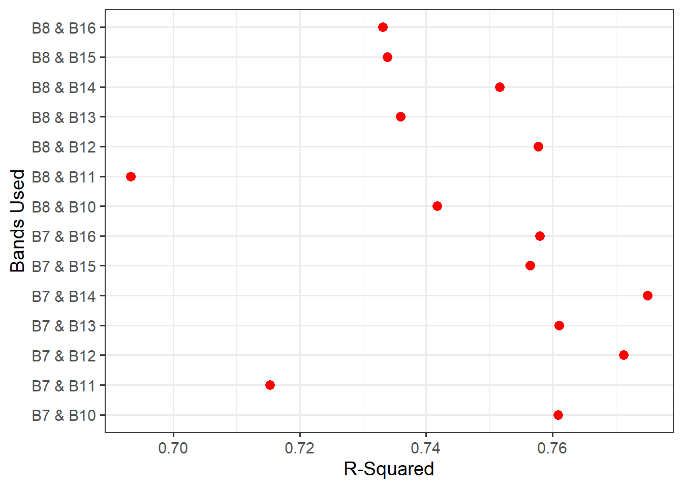
resultsDF |> ggplot(aes(x=rmse, y=case))+
  geom_point(size=3, color="red")+
  theme_bw(base_size=14)+
  labs(x="RMSE", y = "Bands Used")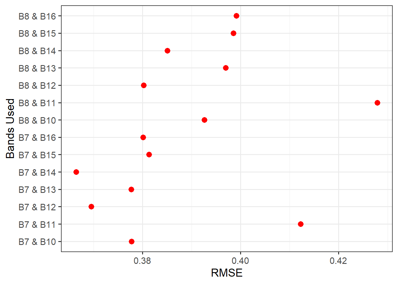
burnR |> ggplot(aes(x=dnbr7_14, y=Total))+
  geom_point(size=2, color="red")+
  geom_smooth(method="lm")+
  theme_bw(base_size=14)+
  labs(x="dNBR (NIR1 and SWIR5)", y="CBI")+
  scale_y_continuous(breaks=seq(0, 3.5, .5))+
  scale_x_continuous(breaks=seq(-1.5, 2, .25))+
  theme(axis.text = element_text(color="black"))+
  theme(axis.title = element_text(color="black"))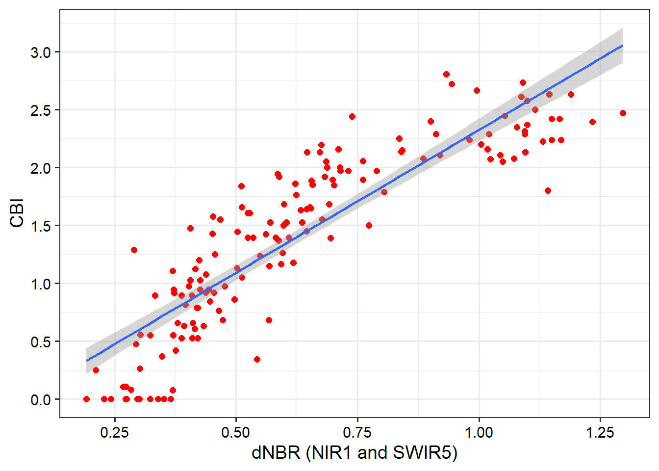
6.3.2 Step-Wise Regression
Now that we have implemented single linear regression, we will explore some augmentations. You may have noticed in the scatter plot generated above when using SWIR Band 14 and NIR Band 7 that the relationship, though generally strong, is not linear. Thus, using a linear model, which is represented as a line, is likely not optimal.
Step-wise regression consists of building a linear model as a series of horizontal line segments with break points between the segments. This type of regression can be implemented using lm() and cut() within the model formula. We specifically use cut points every 0.2 units between 0 and 1.5. We then predict to a new sequence of dNBR values using the predict() function. The resulting model is visualized using ggplot2() and, as the name implies, consists of a series of horizontal line segments or steps.
breaks = seq(0,1.5, .2)
step.new4 = lm(Total ~ cut(dnbr7_14, breaks = breaks), data=burnR)

testValues <- seq(.2, 1.3, .005)
testPred <- predict(step.new4, data.frame(dnbr7_14=testValues))
testOut <- data.frame(pred=testPred, truth=testValues)

burnR$step <- step.new4$fitted.valuesggplot()+
geom_point(data=burnR, aes(x=dnbr7_14, y=Total), size=2, color="red")+
geom_line(data=testOut, aes(y=testPred, x=truth), color="black", lwd=1.5)+
theme_bw(base_size=14)+
labs(x="dNBR", y="Composite Burn Index")+
scale_y_continuous(breaks=seq(0, 3.5, .5))+
scale_x_continuous(breaks=seq(-1.5, 2, .25))+
theme(axis.text = element_text(color="black"))+
theme(axis.title = element_text(color="black"))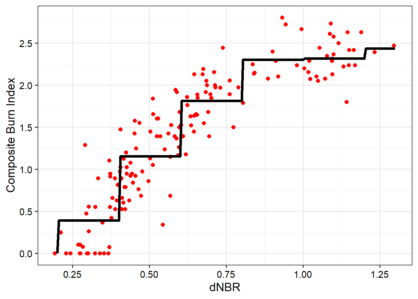
6.3.3 Polynomial Regression
Polynomial regression incorporates the predictor variable raised to a power, commonly either two or three. There is still only one predictor variable; we are simply representing it as two components. The relationship is modeled as follows:
\[
\begin{aligned}
y &= \beta_0
+ \beta_1 x
+ \beta_2 x^{2}
+ \varepsilon
\\[1em]
\text{where}\\
y &\text{ = dependent variable}\\
x_n &\text{ = predictor variable}\\
\beta_0 &\text{ = } \mathit{y} \text{-intercept term} \\
\beta_1 &\text{ = 1st order coefficient for variable } x\\
\beta_2 &\text{ = 2nd order coefficient for variable } x\\
\varepsilon &\text{ = error term (residual)}
\end{aligned}
\] The poly() function implements both the original and higher order terms for the predictor variable. In our example, we are only using orders of one and two. The important point here is that incorporating a square term allows us to model a non-linear relationship with a linear equation. This is still considered a linear model since the relationship is linear in regards to the trainable parameters: coefficients and single y-intercept term.
After fitting the model, we apply it to the data using predict() then plot the results. The polynomial model is able to better capture the non-linear relationship between CBI and dNBR as suggested by the scatter plot. Calculating R-squared and RMSE for this model suggests a better fit (i.e., reduced RMSE and increased R-squared) compared to not incorporating a square term.
The model could also be defined as follows:
lm7_14P <- lm(Total ~ dnbr7_14 + dnbr7_14^2, data=burnR)
or
lm7_14P <- lm(Total ~ dnbr7_14 + (dnbr7_14*dnbr7_14), data=burnR)
Call:
lm(formula = Total ~ poly(dnbr7_14, 2), data = burnR)

Residuals:
     Min       1Q   Median       3Q      Max
-1.01742 -0.18043 -0.02334  0.18578  1.01867

Coefficients:
                   Estimate Std. Error t value Pr(>|t|)
(Intercept)          1.4193     0.0237  59.887   <2e-16 ***
poly(dnbr7_14, 2)1   8.4952     0.2960  28.699   <2e-16 ***
poly(dnbr7_14, 2)2  -2.7465     0.2960  -9.278   <2e-16 ***
---
Signif. codes:  0 '***' 0.001 '**' 0.01 '*' 0.05 '.' 0.1 ' ' 1

Residual standard error: 0.296 on 153 degrees of freedom
Multiple R-squared:  0.856, Adjusted R-squared:  0.8542
F-statistic: 454.9 on 2 and 153 DF, p-value: < 2.2e-16burnR$polyPred <- predict(lm7_14P, burnR)
burnR |> ggplot(aes(x=dnbr7_14, y=Total))+
geom_point(size=2, color="red")+
geom_line(aes(y=polyPred), lwd=1.5, color="black")+
theme_bw(base_size=14)+
labs(x="dNBR", y="Composite Burn Index")+
scale_y_continuous(breaks=seq(0, 3.5, .5))+
scale_x_continuous(breaks=seq(-1.5, 2, .25))+
theme(axis.text = element_text(color="black"))+
theme(axis.title = element_text(color="black"))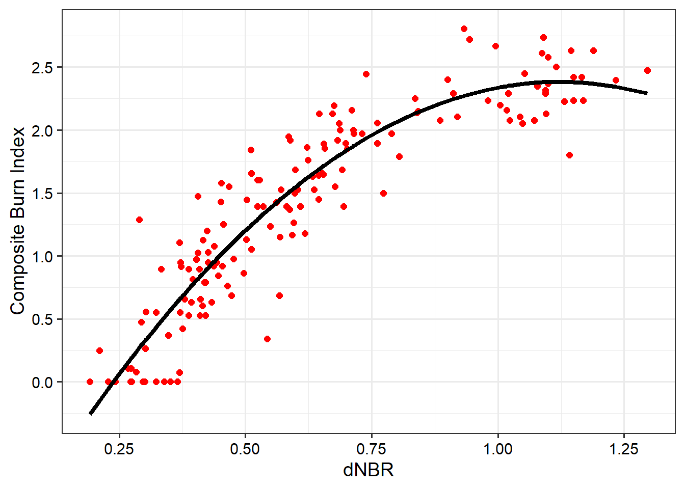
6.4 Using Multiple Predictor Variables
6.4.1 Multiple Linear Regression
In contrast to single or simple linear regression, multiple linear regression incorporates more than one predictor variable. It is also possible to incorporate polynomial terms for all or some of the input predictor variables or some linear combination of them. It is also possible to incorporate interactions, which are discussed below.
\[ \begin{aligned} y &= \beta_0 + \beta_1 x_1 + \beta_2 x_2 + \cdots + \beta_p x_p + \varepsilon \\ \text{where:} \\ y &\text{ = dependent variable} \\ x_p &\text{ = predictor variable } \mathit{p} \\ \beta_0 &\text{ = } \mathit{y} \text{-intercept term} \\ \beta_p &\text{ = slope or coefficient for variable } \mathit{p} \\ \varepsilon &\text{ = error term (residual)} \end{aligned} \]
Our example data are more appropriate for single regression; however, we will re-frame the problem for the purposes of this demonstration by attempting to predict CBI using the change in image band values between the post- and pre-fire values as opposed to dNBR. This requires augmenting the original data by calculating all band differences using dplyr and creating a new tibble (burnDiff) that includes only the CBI (“Total”) data and all differenced bands.
burnDiff <- burn |>
  mutate(blue= (ApB2-DcB2),
         green= (ApB3-DcB3),
         yellow= (ApB4-DcB4),
         red= (ApB5-DcB5),
         redEdge= (ApB6-DcB6),
         nir1= (ApB7-DcB7),
         nir2= (ApB8-DcB8),
         swir1= (ApB9-DcB9),
         swir2= (ApB10-DcB10),
         swir3= (ApB11-DcB11),
         swir4= (ApB12-DcB12),
         swir5= (ApB13-DcB13),
         swir6= (ApB14-DcB14),
         swir7= (ApB15-DcB15),
         swir8= (ApB15-DcB16)) |>
  select(Total,blue,green,
         yellow,red,redEdge,
         nir1,nir2,
         swir1,swir2,swir3,swir4,swir5,swir6,swir7,swir8)
We first fit a model using the NIR and SWIR bands that provided the best result above: NIR1 and SWIR6. To incorporate multiple predictor variables, we use an addition sign in the formula syntax: lm(Total~nir1+swir6, data=burnDiff).
modelMLR <- lm(Total~nir1+swir6, data=burnDiff)We need to visualize the model output differently now that we have two predictor variables. We display the model as a continuous color gradient within the two-dimensional feature space. To accomplish this, we map the NIR1 data to the x-axis position and the SWIR6 data to the y-axis position. The predicted values are shown using the color gradient. This requires making predictions across the range of NIR1 and SWIR6 values. We accomplish this by generating pairs of NIR1 and SWIR6 values using expand.grid() and seq() followed by making predictions using these value combinations with predict(). The visualization is generated using ggplot2() with the geom_tile() geometry. As the visualization suggests, higher burn severity is associated with higher values of SWIR and lower values of NIR reflectance.
testSet <- expand.grid(nir1=seq(-1500, 500, 10),
                       swir6=seq(250, 1500, 10))

predictSet <- predict(modelMLR, testSet)

testSet$pred <- predictSet

ggplot() +
  geom_tile(data = testSet, aes(x = nir1,
                                y = swir6,
                                fill = pred))+
  labs(x = "Change in NIR 1",
       y = "Change in SWIR 6",
       fill = "CBI")+
  scale_fill_gradient(low = "white",
                      high = "red") +
  theme_bw(base_size=14)+
  scale_y_continuous(expand=c(0,0),
                     breaks=seq(250,1500,250))+
  scale_x_continuous(expand=c(0,0),
                     breaks=seq(-1500,500,250))+
  theme(axis.text = element_text(color="black"))+
  theme(axis.title = element_text(color="black"))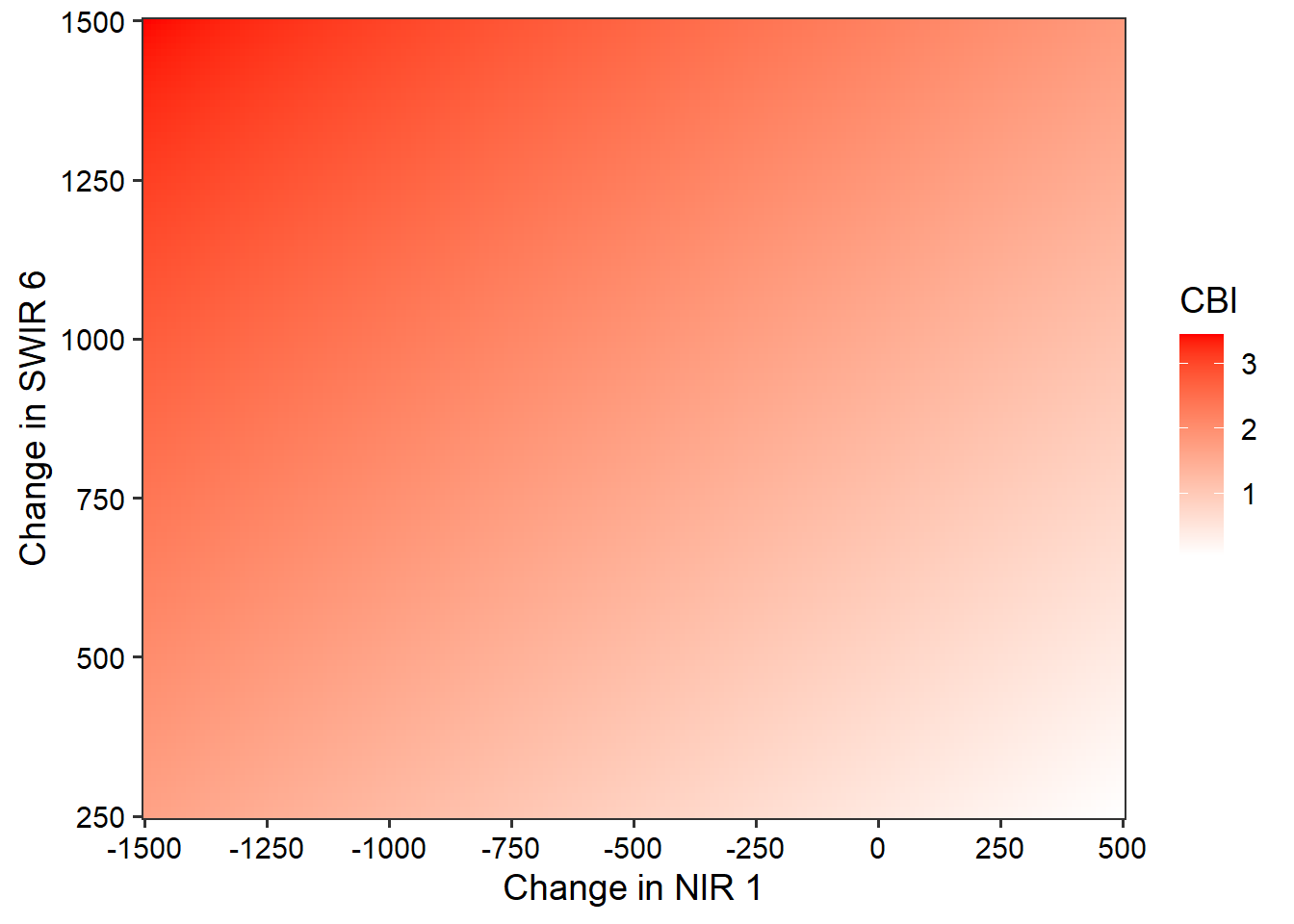
We next produce a model using all channel differences. Printing the model summary, we can see that coefficients have been estimated for each differenced band. If model assumptions are met, these coefficients are generally interpreted as the change in the dependent variable, in this case CBI, for a unit change in the predictor variable associated with the coefficient when holding all other predictor variables constant. The associated t-value is used to assess whether the coefficient is statistically significant. In this model many of the coefficients are not statistically significant. When incorporating polynomial terms and/or interactions, it is important to consider all predictors that include a variable of interest when interpreting coefficients or assessing the relationship between the dependent variable and the predictor variable of interest.
#Plot scatterplots for all band differences and total CBI
custom_labeller <- function(variable, value) {
  # Define the mapping of old to new labels
  label_mapping <- c(
    "blue" = "Blue",
           "green"="Green",
           "yellow"="Yellow",
           "red"="Red",
           "redEdge"="Red Edge",
           "nir1"="NIR1",
           "nir2"="NIR2",
           "swir1"="SWIR1",
           "swir2"="SWIR2",
           "swir3"="SWIR3",
           "swir4"="SWIR4",
           "swir5"="SWIR5",
           "swir6"="SWIR6",
           "swir7"="SWIR7",
           "swir8"="SWIR8"
  )
  # Return the new label based on the mapping
  return(label_mapping[value])
}
burnDiff |>
melt(id="Total") |>
ggplot(aes(x=value, y=Total))+
geom_point(color="#444444", size=2, color="red")+
facet_wrap(vars(variable), ncol=5,
labeller = labeller(variable=c(
"blue" = "Blue",
"green"="Green",
"yellow"="Yellow",
"red"="Red",
"redEdge"="Red Edge",
"nir1"="NIR1",
"nir2"="NIR2",
"swir1"="SWIR1",
"swir2"="SWIR2",
"swir3"="SWIR3",
"swir4"="SWIR4",
"swir5"="SWIR5",
"swir6"="SWIR6",
"swir7"="SWIR7",
"swir8"="SWIR8"
)))+
theme_bw(base_size=16)+
labs(x="Pixel value", y="Composite burn index")+
scale_y_continuous(limits=c(0,3), breaks=seq(0,3,1))+
theme(axis.text = element_text(color="black"))+
theme(axis.title = element_text(color="black"))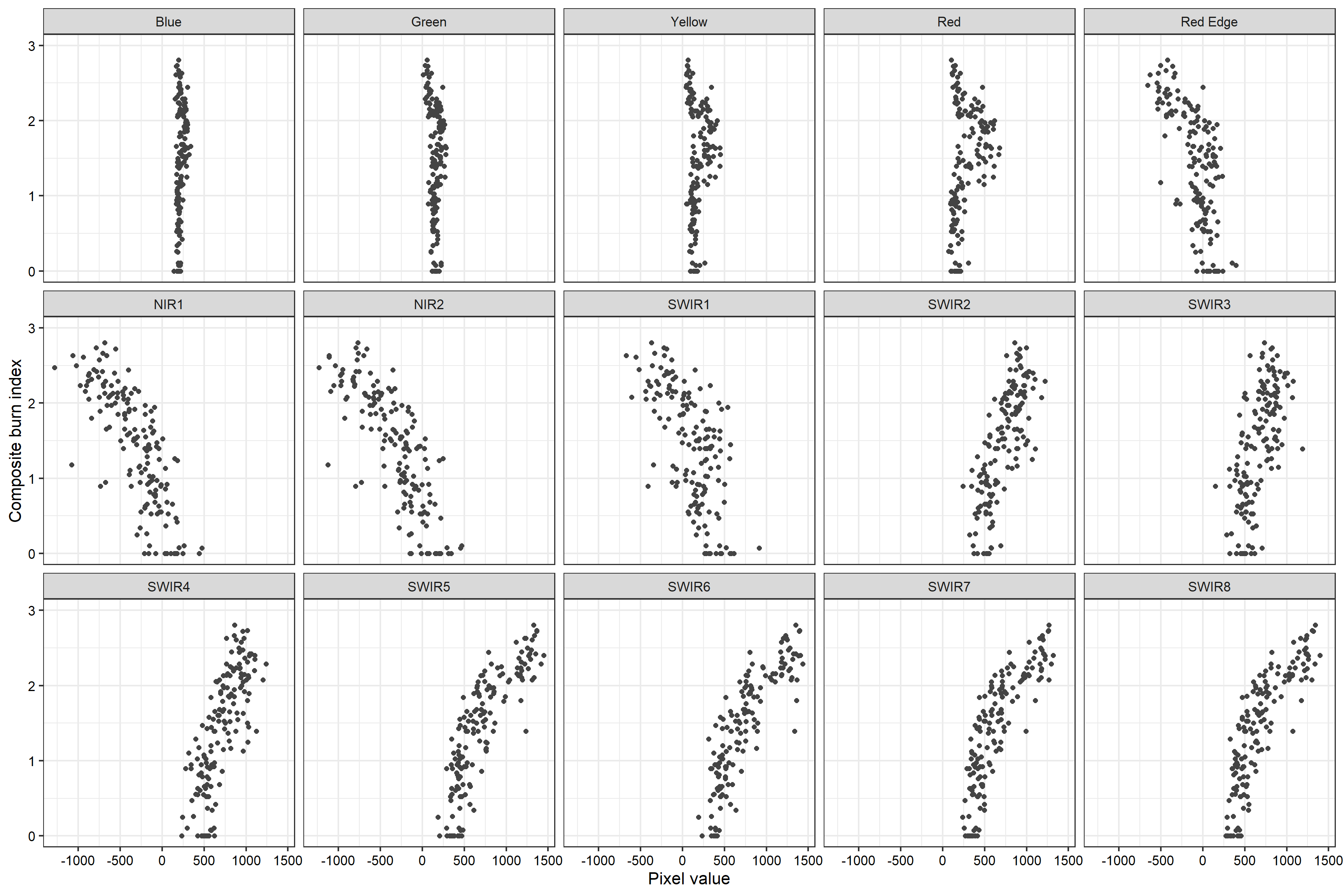
Call:
lm(formula = Total ~ ., data = burnDiff)

Residuals:
     Min       1Q   Median       3Q      Max
-0.63333 -0.18260 -0.00368  0.19850  0.66600

Coefficients:
              Estimate Std. Error t value Pr(>|t|)
(Intercept)  0.1607968  0.2484614   0.647   0.5186
blue         0.0022369  0.0022404   0.998   0.3198
green       -0.0036072  0.0024044  -1.500   0.1358
yellow      -0.0008493  0.0017875  -0.475   0.6354
red          0.0020609  0.0008712   2.366   0.0194 *
redEdge      0.0016164  0.0007505   2.154   0.0330 *
nir1        -0.0003038  0.0004136  -0.735   0.4638
nir2        -0.0010242  0.0004010  -2.554   0.0117 *
swir1       -0.0001497  0.0002394  -0.625   0.5328
swir2       -0.0009375  0.0005756  -1.629   0.1056
swir3       -0.0005527  0.0004637  -1.192   0.2354
swir4        0.0008950  0.0004970   1.801   0.0739 .
swir5        0.0011423  0.0005907   1.934   0.0552 .
swir6        0.0006174  0.0005925   1.042   0.2992
swir7        0.0016493  0.0011596   1.422   0.1572
swir8       -0.0019339  0.0012368  -1.564   0.1201
---
Signif. codes:  0 '***' 0.001 '**' 0.01 '*' 0.05 '.' 0.1 ' ' 1

Residual standard error: 0.2923 on 140 degrees of freedom
Multiple R-squared:  0.8716,    Adjusted R-squared:  0.8578
F-statistic: 63.35 on 15 and 140 DF,  p-value: < 2.2e-16
6.4.2 Incorporating Interactions
Interaction terms can be useful when the response of the dependent variable to predictor variable A changes with values of predictor variable B and vice versa. Interaction terms are not meant to model correlation between the two predictor variables, which is a common misconception.
Incorporating interactions terms can be accomplished with :. In the example below, we are attempting to predict CBI using the NIR1 and SWIR6 bands along with their interaction. It is also possible to incorporate polynomial terms and interactions, as demonstrated in the second example.
When performing feature selection, if the coefficient for the interaction term between two predictor variables is statistically significant but one or both coefficients for the predictor variables are not statistically significant, it is common practice to still include the single predictor variables. In other words, if an interaction term is included in a model the individual variables used within it should also be included.
Call:
lm(formula = Total ~ nir1 + swir6 + nir1:swir6, data = burnDiff)

Residuals:
     Min       1Q   Median       3Q      Max
-1.17295 -0.20410  0.02359  0.23525  0.86262

Coefficients:
              Estimate Std. Error t value Pr(>|t|)
(Intercept) -3.585e-01  1.039e-01  -3.450 0.000726 ***
nir1        -2.054e-03  2.340e-04  -8.779 3.19e-15 ***
swir6        2.215e-03  1.763e-04  12.567  < 2e-16 ***
nir1:swir6   1.681e-06  2.803e-07   5.998 1.40e-08 ***
---
Signif. codes:  0 '***' 0.001 '**' 0.01 '*' 0.05 '.' 0.1 ' ' 1

Residual standard error: 0.3294 on 152 degrees of freedom
Multiple R-squared:  0.8229,    Adjusted R-squared:  0.8194
F-statistic: 235.5 on 3 and 152 DF,  p-value: < 2.2e-16
modelPolyI <- lm7_14P <- lm(Total~poly(nir2,2)+poly(swir6,2)+nir2:swir6, data=burnDiff)
summary(lm7_14P)
Call:
lm(formula = Total ~ poly(nir2, 2) + poly(swir6, 2) + nir2:swir6,
    data = burnDiff)

Residuals:
     Min       1Q   Median       3Q      Max
-1.08087 -0.20013 -0.00481  0.20045  0.76494

Coefficients:
                  Estimate Std. Error t value Pr(>|t|)
(Intercept)      1.370e+00  1.487e-01   9.216 2.60e-16 ***
poly(nir2, 2)1  -2.997e+00  1.507e+00  -1.988   0.0486 *
poly(nir2, 2)2  -1.390e+00  4.624e-01  -3.007   0.0031 **
poly(swir6, 2)1  5.478e+00  9.591e-01   5.712 5.82e-08 ***
poly(swir6, 2)2 -2.007e+00  3.875e-01  -5.180 7.04e-07 ***
nir2:swir6      -1.432e-07  4.287e-07  -0.334   0.7388
---
Signif. codes:  0 '***' 0.001 '**' 0.01 '*' 0.05 '.' 0.1 ' ' 1

Residual standard error: 0.2998 on 150 degrees of freedom
Multiple R-squared:  0.8552,    Adjusted R-squared:  0.8504
F-statistic: 177.2 on 5 and 150 DF,  p-value: < 2.2e-16
6.5 Regression Diagnostics
Linear regression has several assumptions. The key assumptions are as follows:
- The model errors or residuals are normally distributed
- The relationship between the dependent variable and each predictor variable is linear
- The residuals do not vary with predicted dependent variable values (homoscedasticity)
- All samples are independent (i.e., no autocorrelation)
- For multiple linear regression, it is also generally assumed that pairs of predictor variables are not highly correlated
When a linear model will be used to make predictions, as is our primary focus here, as opposed to being used for statistical inference or to understand the correlation or relationship between the dependent variable and each predictor variable, invalid model assumptions are generally less of a concern. Instead, we are more concerned with the accuracy of predictions made for new data (i.e., how well the model generalizes to new data). This is assessed using assessment metrics, such as RMSE, calculated for withheld test samples.
If the relationship between the predictor variables and the dependent variable are not linear and cannot be easily made more linear, such as by including polynomial terms or transforming variables using data transformations, then linear regression may simply not be a good option for this specific predictive modeling task. In such cases, other predictive modeling methods should be considered, such as generalized linear models (GLMs), generalized additive models (GAMs), or machine learning (ML) algorithms.
Even though assessing linear regression model assumptions is less important for predictive modeling tasks, we discuss model assumption assessment here since this is an important component of linear regression in general. For example, if your goal is to quantify whether there is a statistically significant correlation between the dependent variable and a specific predictor variable, you can make use of the t-test results obtained for that specific predictor variable’s coefficient. However, this test is only valid if model assumptions are met. The direction and magnitude of the coefficient for a specific predictor variable is meant to quantify the change in the dependent variable with a one unit change in the dependent variable of interest when holding all other predictor variables constant. If there is multicollinearity between predictor variables, “holding all other predictor variables constant” is really not meaningful since one predictor variable is likely to change when the other variables change.
6.5.1 Normality of Residuals
In our examples, we will make use of our polynomial regression model that used the NIR1 and SWIR6 bands. We recreate the model in the first code block.
The normality of the residuals can be visually assessed by first calculating the residuals then plotting their distribution. In our example, we use a histogram. This could also be accomplished with a kernel density plot.
lm7_14P <- lm(Total~poly(dnbr7_14, 2), data=burnR)
preds <- predict(lm7_14P, burnR)

burnR$pred <- preds

burnR$res <- burnR$Total - preds

burnR |> ggplot(aes(x=res))+
  geom_histogram(binwidth=.05)+
  theme_bw(base_size=14)+
  scale_y_continuous(expand=c(0,0))+
  scale_x_continuous(expand=c(0,0))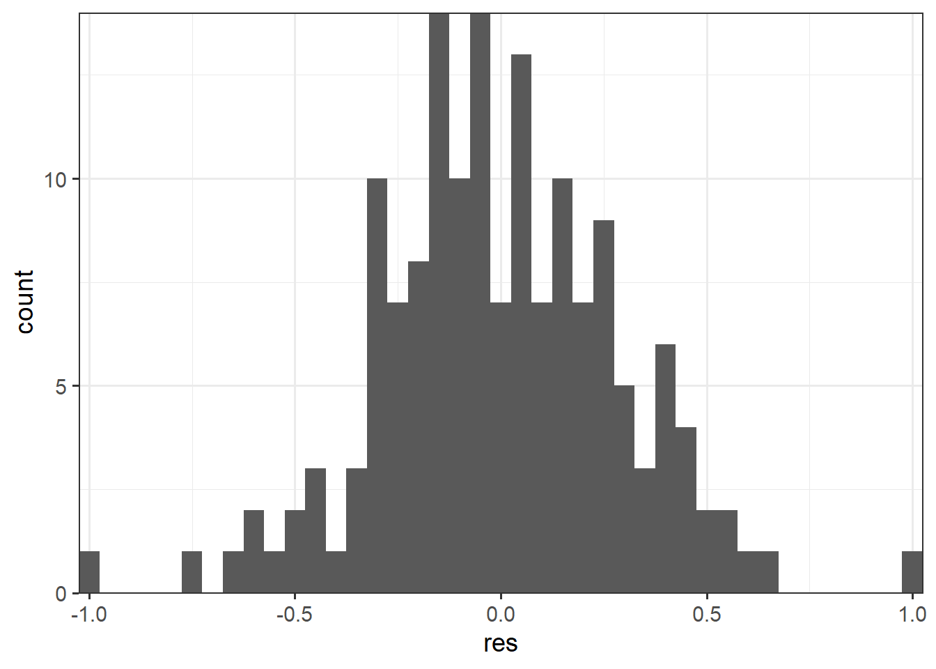
Another option is a quantile-quantile plot (QQ plot). This is a scatter plot where the quantiles of the actual or standardized residuals are plotted to one axis while theoretical quantiles that represent the distribution of the residuals or standardized residuals if they were normally distributed are plotted to the other axis. If the actual and theoretical quantiles are similar, then the data points, which represent individual samples, should generally fall along the one-to-one line. Divergence from this line suggest issues of skewness (i.e., a left- or right-tail), kurtosis (i.e., wider or narrower than a normal distribution), or some other non-normal distribution characteristic.
ggplot() +
  geom_qq(aes(sample = rstandard(lm7_14P))) +
  geom_abline(color = "red") +
  coord_fixed()+
  theme_bw(base_size=14)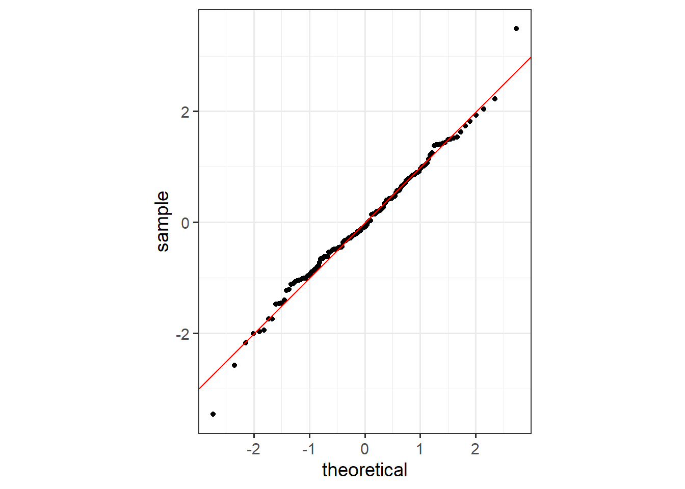
The Shapiro-Wilk Normality Test is a statistical test of normality. The results generally suggest that the residuals are normally distributed or that this assumption is not violated.
shapiro.test(rstandard(lm7_14P))
    Shapiro-Wilk normality test

data:  rstandard(lm7_14P)
W = 0.99054, p-value = 0.3838
6.5.2 Linear Relationships
Linear relationships can be assessed using the Ramsey Regression Equation Specification Error Test (RESET) and visualized by plotting the model residuals against the predictor variable values, which should show a linear trend if there is a linear relationship between the dependent variable and predictor variable of interest.
If there is not a linear relationship, you may considered applying a data transformation, such as Box-Cox, Yeo-Johnson, square root, or logarithmic. Adding polynomial terms may also be useful. If these changes fail to improve the linearity of the relationship, linear regression may not be a good modeling choice for the problem.
The Ramsey RESET test generally suggests that the linearity assumption is met when using polynomial regression to include the second-order term. If only a first order term is used, the RESET test is statistically significant, which suggests that the model assumption is violated. In short, adding the polynomial term here is justified by this result.
resettest(lm7_14P)
    RESET test

data:  lm7_14P
RESET = 1.1464, df1 = 2, df2 = 151, p-value = 0.3205resettest(lm7_14)
    RESET test

data:  lm7_14
RESET = 42.822, df1 = 2, df2 = 152, p-value = 1.777e-15ggplot(burnR, aes(dnbr7_14, res)) +
geom_point() +
geom_hline(yintercept = 0, color = "red") +
geom_smooth()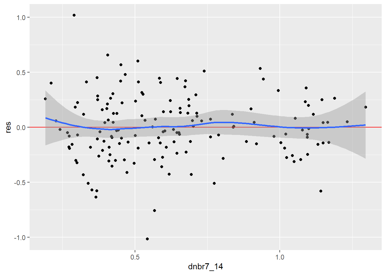
6.5.3 Homoscedasticity
Homoscedasticity suggests that the variability or magnitude of the error or residuals do not change with predicted values of the dependent variable. In other words, the model should do an equally good or bad job predicting the dependent variable despite its values. This can be visually assessed by using a scatter plot where the predicted dependent variable values are plotted to the x-axis and the residuals are plotted to the y-axis.
Homoscedasticity is suggested when the pattern is random or there is no change in residual magnitude with predicted values of the dependent variable. If there are patterns, this suggests heteroscedasticity. For example, a greater magnitude of model errors when predicted dependent variable values are larger suggests that the model is doing a poorer job predicting larger values of the dependent variable in comparison to smaller values. These plots can also be helpful for assessing for model bias. For example, if residuals are negative at lower values of the predicted dependent variable but positive at larger predicted dependent variable values, this indicates that the model is under-predicting low values and over-predicting high values.
The Non-Constant Variance Score (NCV) Test can also assess for heteroscedasticity issues. For our example, the plot suggests that there might be an issue with this assumption, but it in unclear. However, the NCV test suggests this assumption is violated since the test yields a statistically significant result.
burnR |> ggplot(aes(x=pred, y=res))+
  geom_point(color="red", size=2)+
  geom_hline(yintercept=0, lwd= 1.5, linetype=2)+
  theme_bw(base_size=14)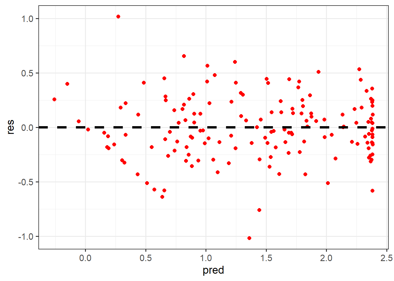
ncvTest(lm7_14P)Non-constant Variance Score Test
Variance formula: ~ fitted.values
Chisquare = 5.098371, Df = 1, p = 0.0239486.5.4 Multicollinearity
Multicollinearity, or correlation between predictor variables, can be visualized using individual scatter plots for pairs of predictor variables, a scatter plot matrix, or a correlation matrix. The corrplot package is excellent for generating correlation matrices. Another option is the variable inflation factor (VIF) metric. A commonly used VIF threshold that suggests multicollinearity is if the square root of VIF is larger than two for the pair of predictor variables.
If issues of multicollinearity are discovered, this generally suggests that the coefficients and associated statistical tests may be misleading or flawed. If this is not a major concern, such as for predictive modeling, multicollinearity is generally less of a concern.
For our model that incorporated all band differences (modelMLR), the results below suggest issues of multicollinearity. The scatter plot matrix suggests strong correlation between predictor variables and some VIF values are high.
M = burnDiff |> select(-Total) |> cor()
corrplot.mixed(M)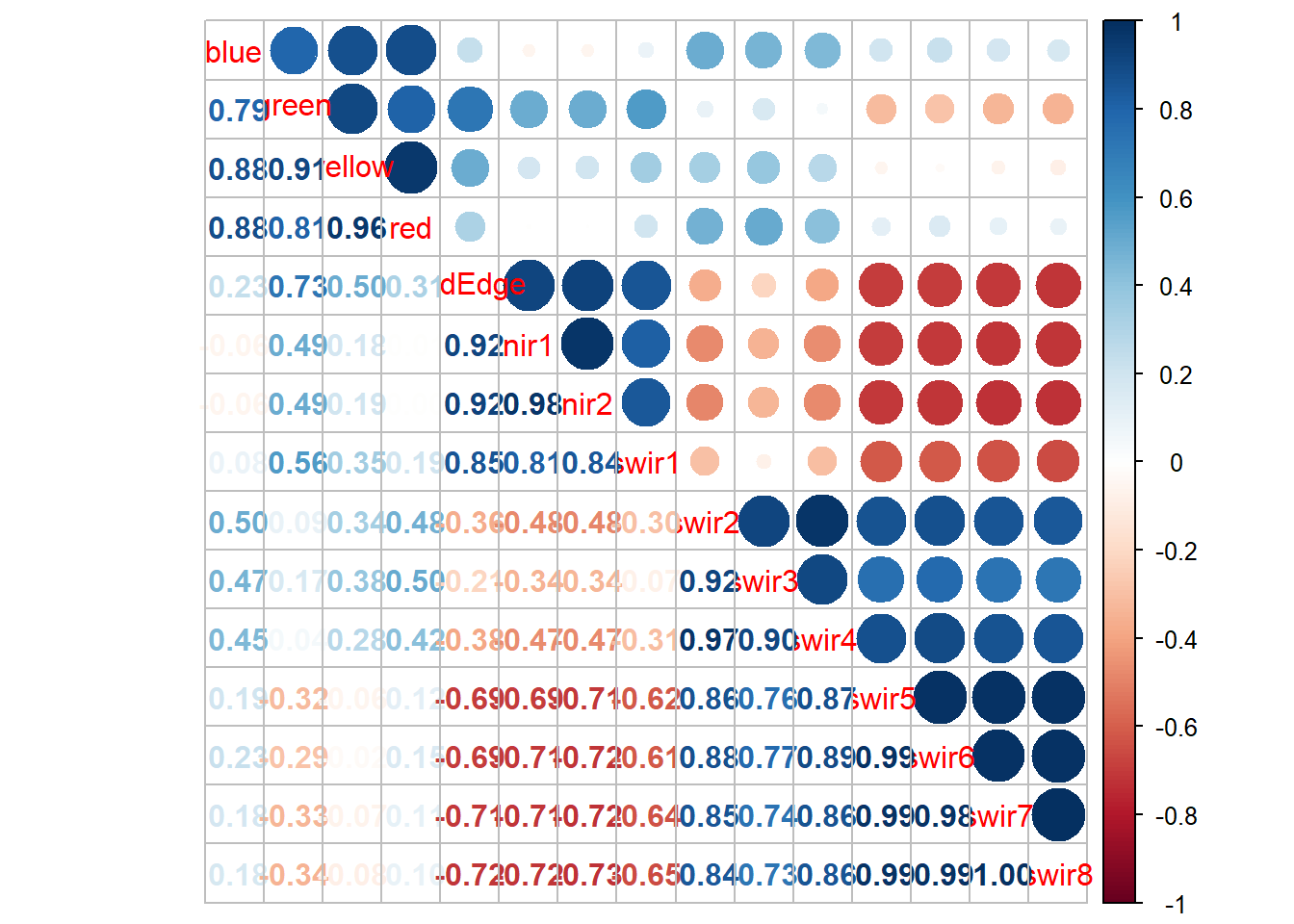
vif(modelMLR) blue green yellow red redEdge nir1 nir2
14.495852 34.960424 58.652994 33.675912 48.196500 34.932839 39.035599
swir1 swir2 swir3 swir4 swir5 swir6 swir7
8.596339 26.697439 13.915205 22.103095 67.779113 68.854112 220.681876
swir8
259.004627 blue green yellow red redEdge nir1 nir2 swir1 swir2 swir3
TRUE TRUE TRUE TRUE TRUE TRUE TRUE TRUE TRUE TRUE
swir4 swir5 swir6 swir7 swir8
TRUE TRUE TRUE TRUE TRUE 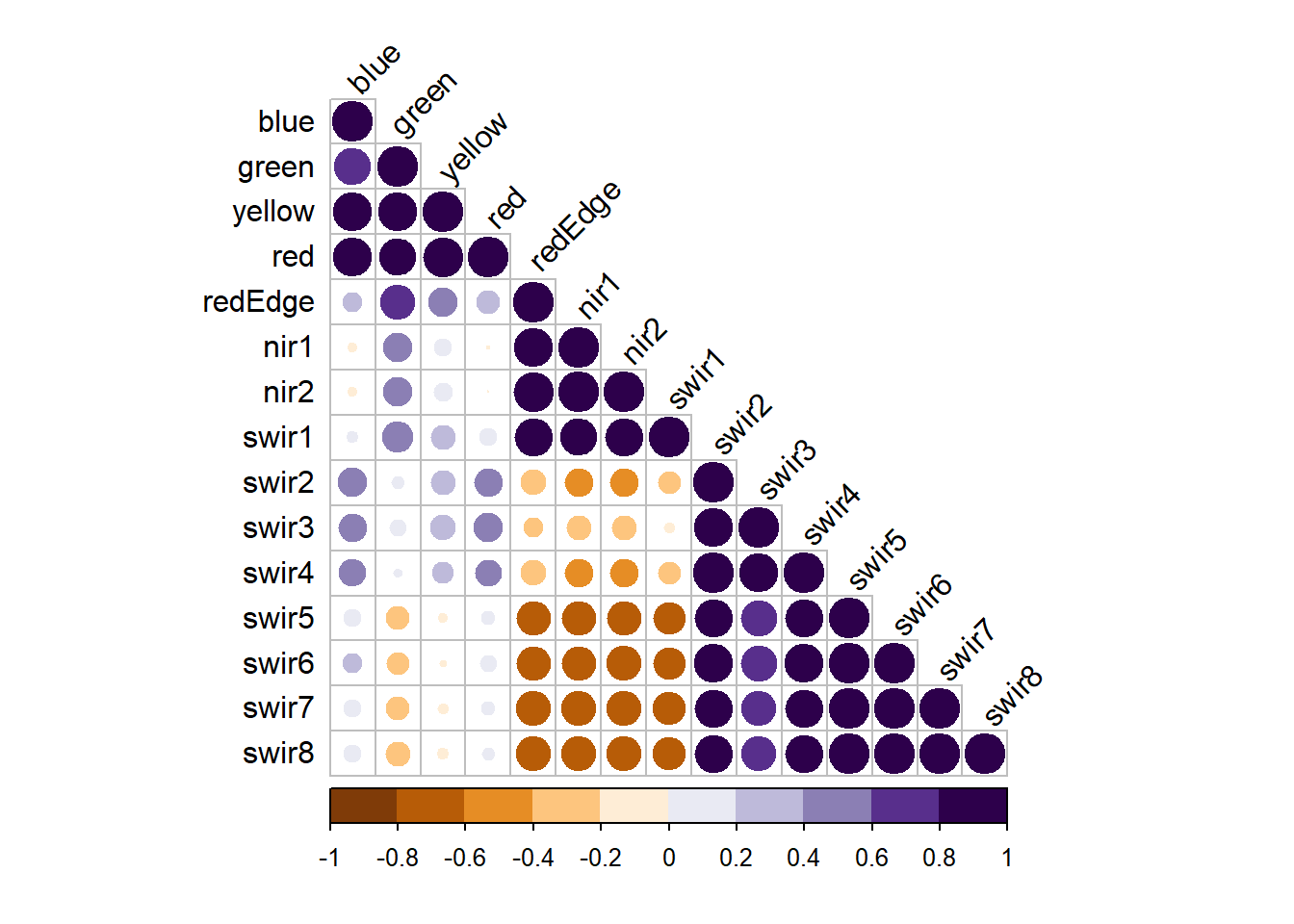
6.5.5 Other Concerns
In regards to autocorrelation, for spatial data we are generally most concerned with spatial autocorrelation. This is commonly assessed using the Moran’s I statistic. We generally consider spatial autocorrelation of the dependent variable values or the model residuals. This metric can be calculated using the spdep package.
Correlation through time, or for nearer records in a data table, can be assessed with the Durbin-Watson Test, which is implemented in the car package.
6.6 Regularization
In order to reduce overfitting or improve model generalization, regularization can be implemented. Common methods include ridge regression, which uses L2 regularization, or lasso regression, which uses L1 regularization. Both methods penalize a model for having larger model coefficients. L2 regularization uses the square root of the coefficients, so it is not possible for the coefficients to decrease to zero. In contrast, L1 regularization penalizes based on the absolute value of the coefficients; as a result, it is possible for predictor variables to drop out of the model when using lasso regression but not ridge regression since their association coefficients can be reduced to zero. As a result, lasso regression is sometimes used as a feature selection method.
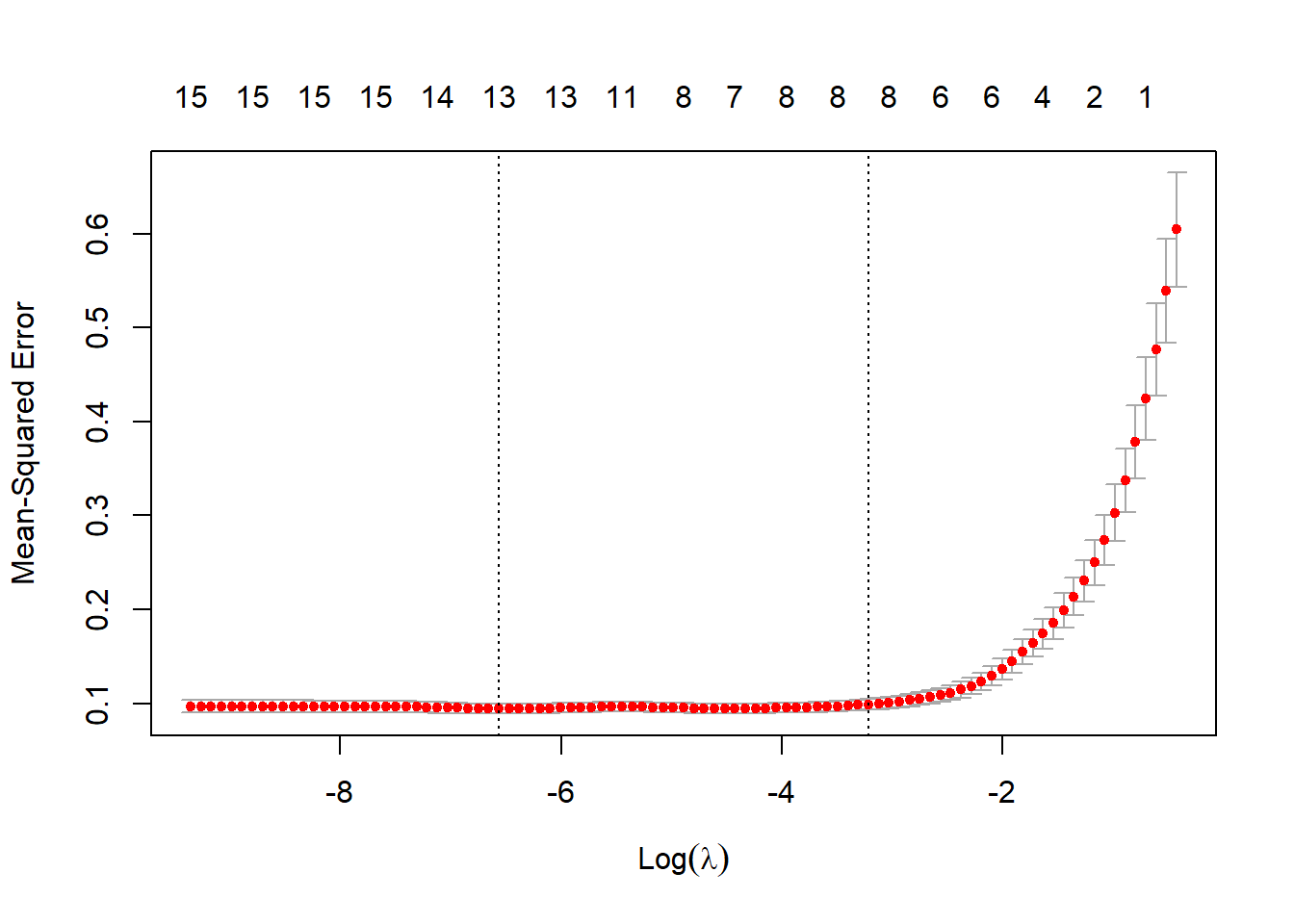
The code below demonstrates how to implement lasso regression in R using the glmnet package. This involves (1) converting the input data to R matrices and separating the predictor variables and dependent variable into separate objects, (2) selecting a lambda value via a cross validation process, and (3) fitting the model with the selected lambda value. Lambda is a lasso regression hyperparameter that impacts the degree of penalization applied. Since the optimal degree of penalization is not known beforehand, it is generally recommended that lambda be tuned.
16 x 1 sparse Matrix of class "dgCMatrix"
                       s0
(Intercept)  0.0190688095
blue         0.0019988362
green       -0.0034096249
yellow       .
red          0.0017061398
redEdge      0.0009183705
nir1        -0.0001409784
nir2        -0.0008983867
swir1       -0.0001814943
swir2       -0.0006198924
swir3       -0.0003400899
swir4        0.0008202789
swir5        0.0008405812
swir6        0.0001753322
swir7        0.0001658775
swir8        .
6.7 Predict to Raster Data
Lastly, we want to demonstrate how a linear regression model can be used to make spatial predictions on a cell-by-cell basis. We first read in the pre- and post-fire images. The values from the table used throughout this chapter are from these images. The images are then displayed as false color composites using the SWIR6, NIR1, and green channels. In the second image, the extent of the fire is obvious using this band composite, which highlights the value of SWIR and NIR data for mapping fire extents and fire severity.
preImg |> plotRGB(r=14,g=7,b=3, stretch="lin")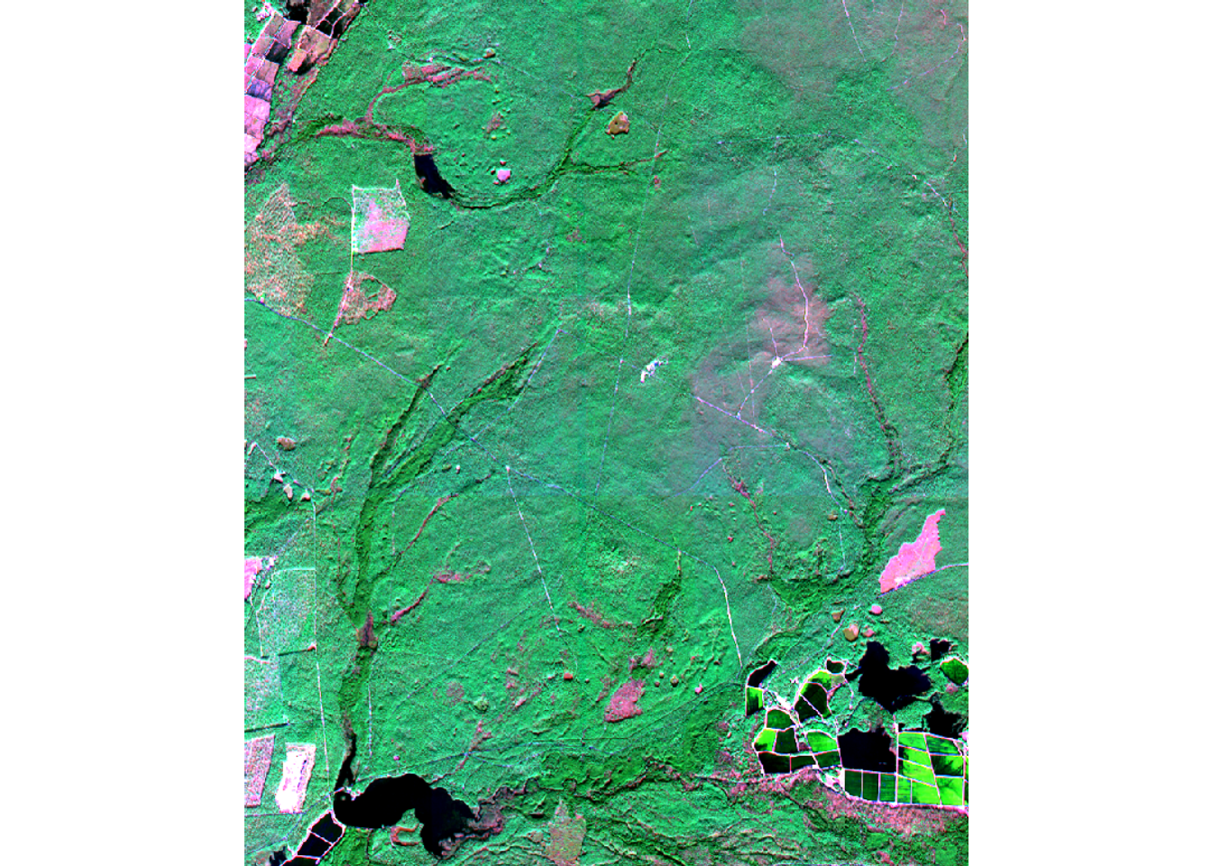
postImg |> plotRGB(r=14,g=7,b=3, stretch="lin")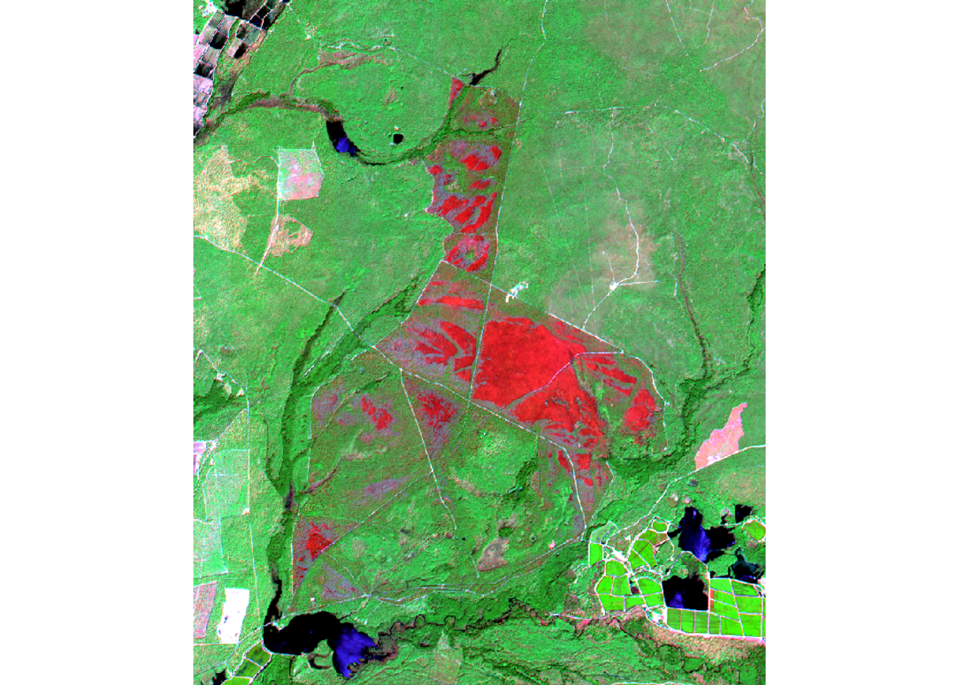
Next, we generate the dNBR that was selected as optimal above (i.e., NIR1 and SWIR6), calculate NBR for each image, then use the results to calculated dNBR on a pixel-by-pixel basis. We now have the single predictor variable used in our linear model as a raster grid.
Any preprocessing applied to the tabulated data must also be applied to the image data so that the cell values match those used in the modeling. No preprocessing was applied here, so we do not need to worry about this.
nir2Pre <- preImg |> subset(7)
nir2Post <- postImg |> subset(7)
swir6Pre <- preImg |> subset(14)
swir6Post <- postImg |> subset(14)

nbrPre <- (nir2Pre-swir6Pre)/(nir2Pre+swir6Pre)
nbrPost <- (nir2Post-swir6Post)/(nir2Post+swir6Post)
nbrPost <- resample(nbrPost, nbrPre)

dnbrR <- nbrPre-nbrPost
dnbrR <- clamp(dnbrR, lower=-2, upper=2)tm_shape(dnbrR)+
tm_raster(col.scale = tm_scale_intervals(style= "quantile",
n=7,
values="brewer.reds"),
col.legend = tm_legend(title = "dNBR"))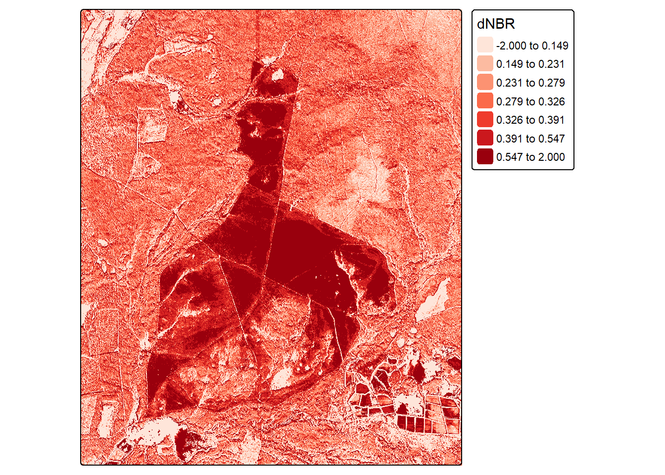
Since our model consists of learned coefficients, we can apply it using simple raster math. We are specifically creating a prediction using the polynomial single regression equation. The learned coefficient for the dNBR variable is multiplied by each cell value. We add to this the square term coefficient multiplied by the square of the dNBR at each pixel. Lastly, we add the y-intercept. Note that this model could also be applied using the predict() function. In later chapters, we will generally make use of this function for applying our models to new data tables or raster grid cells since the models will be too complex to apply using simple raster math.
The resulting prediction is plotted using tmap. If desired, this prediction can be saved to disk using writeRaster() from terra as a single-band raster grid.
summary(lm7_14P)
Call:
lm(formula = Total ~ poly(dnbr7_14, 2), data = burnR)

Residuals:
     Min       1Q   Median       3Q      Max
-1.01742 -0.18043 -0.02334  0.18578  1.01867

Coefficients:
                   Estimate Std. Error t value Pr(>|t|)
(Intercept)          1.4193     0.0237  59.887   <2e-16 ***
poly(dnbr7_14, 2)1   8.4952     0.2960  28.699   <2e-16 ***
poly(dnbr7_14, 2)2  -2.7465     0.2960  -9.278   <2e-16 ***
---
Signif. codes:  0 '***' 0.001 '**' 0.01 '*' 0.05 '.' 0.1 ' ' 1

Residual standard error: 0.296 on 153 degrees of freedom
Multiple R-squared:  0.856, Adjusted R-squared:  0.8542
F-statistic: 454.9 on 2 and 153 DF,  p-value: < 2.2e-16
cbiR <- (8.4952*dnbrR)+ (-2.7465*(dnbrR*dnbrR)) + 1.4193tm_shape(cbiR)+
tm_raster(col.scale = tm_scale_intervals(style= "quantile",
n=7,
values="brewer.reds"),
col.legend = tm_legend(title = "CBI"))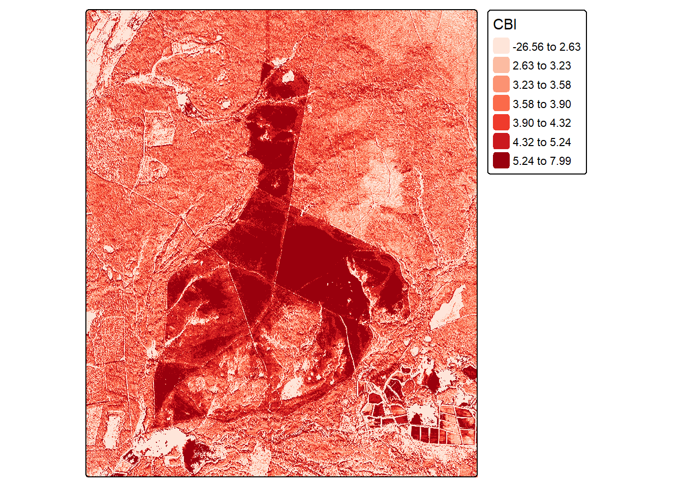
6.8 Concluding Remarks
This chapter focused on conducting linear regression in R using predominantly base R functionality. We explored how to build both single and multiple regression models and incorporate higher order terms and interactions. Models were assessed and compared using RMSE and R-squared values. We also discussed how to perform some linear regression assumption diagnostics using graphs/visualizations and also statistical tests. We explored how to implement lasso regression, which makes use of L1 regularization, which can aid in reducing overfitting and/or to perform variable selection. Lastly, we applied our polynomial regression model to a grid of dNBR values derived from pre- and post-fire WorldView-3 images on a cell-by-cell basis to obtain a spatial prediction.
Now we are ready to investigate additional supervised learning methods, which generally have a similar workflow to linear regression. In the next chapter, we explore spatial probabilistic mapping using the random forest algorithm. The rest of this section explores the tidymodels framework for implementing ML using a common syntax.
6.9 Questions
- Why is polynomial regression still considered a linear model when the modeled relationship can have curvature?
- Explain the concept of homoscedasticity.
- How is the variable inflation factor (VIF) calculated?
- Explain the difference between a linear model, a generalized linear model, and a generalized additive model.
- Explain the difference between ridge regression, lasso regression, and elastic net.
- What is the purpose of the Moran’s I statistic?
- Assuming model assumptions are met, explain how to interpret the coefficient or slope term associated with a single predictor variable in multiple linear regression.
- Explain the use and interpretation of the Shapiro-Wilk Test and how it is calculated.
6.10 Exercises
You will now further explore the CBI prediction problem presented in this chapter by fitting a generalized additive model (GAM) and comparing it to the linear and polynomial models generated above. Use SWIR6 (Band 14) and NIR1 (Band 7) for this analysis. Complete the following tasks.
- Randomly split the data so that 100 samples are used for training and the remaining samples are withheld for testing. This can be accomplished using dplyr or rsample.
- Calculate the dNBR using SWIR6 (Band 14) and NIR1 (Band 7).
- Fit the linear model (
cbi ~ dNBR) and polynomial model (cbi ~ dNBR + dNBR^2) using the training subset. - Fit a GAM to predict CBI using the dNBR and the training subset. This can be accomplished using the
gam()function from the mgcv package. Usefamily = gaussian(). - Use all three models to predict the withheld test data.
- Use the predictions and the CBI measures for the test data to calculate the RMSE and predicted R-squared for each model.
- Write a paragraph describing your results. Which model generalized the best to the withheld test data? Did the GAM overfit in comparison to the other two models?