15 Geospatial Semantic Segmentation
15.1 Topics Covered
- Understand the general geodl workflow
- Generate raster masks or labels from input vector data
- Generate chips and associated masks and list them into a data frame
- Define a torch dataset with optional data augmentations
- Check and visualize data prior to training a model
- Define a UNet, UNet with a MobileNetv2 encoder, UNet3+, or HRNet architecture for semantic segmentation
- Configure losses using the unified focal loss framework
- Assess models using point or pixel locations, raster grids, or a torch DataLoader.
- Generate land surface parameters (LSPs) using GPU-based computation
- Configure a model for extracting landforms or geomorphic features from LSP predictor variables
15.2 Introduction
The geodl R package supports semantic segmentation, or pixel-level classification, in R. It builds on torch and luz, which support the deep learning (DL) component, and terra, which is used for reading and processing geospatial raster data. This package was created by the author’s of this text and was introduced in the following paper:
Maxwell, A.E., Farhadpour, S., Das, S. and Yang, Y., 2024. geodl: An R package for geospatial deep learning semantic segmentation using torch and terra. PloS one, 19(12), p.e0315127.
Since the release of this paper, geodl has been expanded to include more semantic segmentation models, training routines that do not require generating image chips beforehand, and additional functionality for generating land surface parameters (LSPs) and performing DL using LSP predictor variables.
In this first chapter focused on geodl, we provide a detailed discussion of the package design and associated workflows. In the following chapter, we demonstrate three semantic segmentation workflows. Our goal is to provide background information and demonstrate workflows so that you have a working knowledge of the package and its underlying philosophy and can modify example workflows to meet your own needs.
geodl is still actively being developed. We recommend installing it from GitHub as opposed to CRAN. This can be accomplished using devtools as follows:
devtools::install_github("maxwell-geospatial/geodl")
15.2.1 Semantic Segmentation
In contrast to scene classification or scene labeling, which was explored in the first three chapters of this section, semantic segmentation entails pixel-level as opposed to scene-level labeling. This is generally a more difficult task due to increases in class heterogeneity and complex class signatures. However, it has a wide variety of use cases in remote sensing and the geospatial sciences. For example, semantic segmentation can be used to generate land cover maps and differentiate vegetation community types.
15.2.2 geodl Overview
The goal of geodl is to simplify the task of semantic segmentation using R and torch. It specifically provides tools for:
- Generating raster-based masks or reference labels from vector geospatial data
- Generating image chips from larger extents of input predictor variable raster grids and associated masks
- Training models using pre-generated image chips or chips created dynamically during the training process
- Defining a torch dataset subclass for geospatial data with the ability to apply data augmentations to combat overfitting
- Applying common assessment metrics: overall accuracy, precision, recall, and F1-score
- Implementing the unified focal loss framework after Yeung et al. (2022)
- Defining and training convolutional neural network (CNN) semantic segmentation architectures including a customizable UNet, UNet with a MobileNetv2 encoder, UNet3+, and HRNet (with some modifications from the original implementation)
- Making predictions to full spatial extents to generate both classification and probabilistic output
- Performing assessment using point or pixel locations, raster grids, or a torch dataloader
- Generating LSPs from a DTM using torch and GPU-based computation
- Implementing a semantic segmentation model designed specifically for geomorphic or landform feature extraction tasks
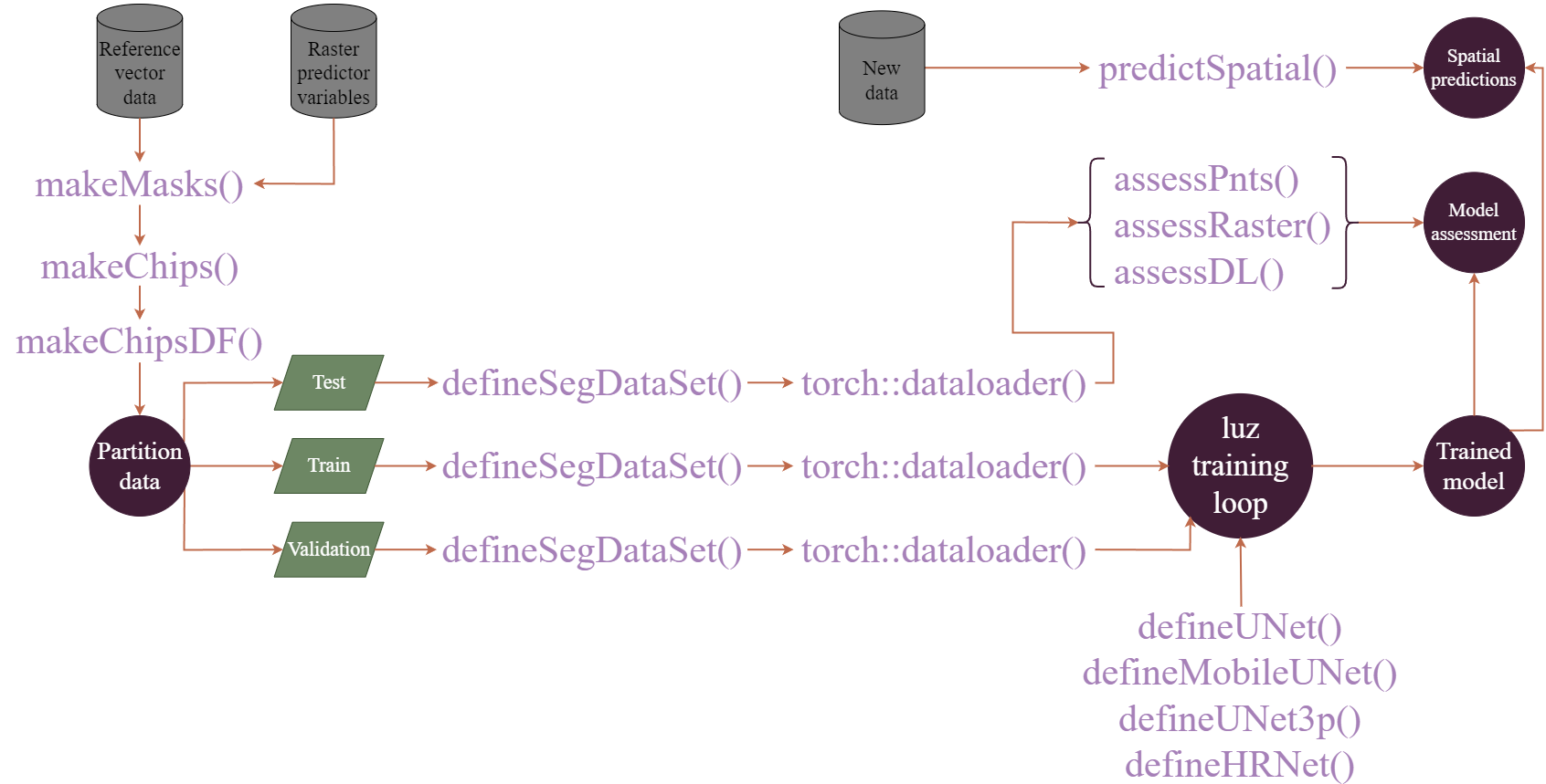
Simplified workflows are shown in Figure 15.1 and Figure 15.2. The first figure demonstrates the process when image chips are generated prior to the training process. The makeMasks() function allows for generating raster masks or labels from input vector geospatial data that align with input raster-based predictor variables. This results in a categorical raster grid where each class is assigned a numeric code. Using the input raster-based predictor variables and generated raster masks, the makeChips() or makeChipsMultiClass() function creates image chips and associated masks that are written to disk to a user-defined directory. The generated image chip size is defined by the user. The chip and mask paths can then be written into a data frame using the makeChipsDF() function.
In torch, the dataset class defines how input data are processed to generate a single example tensor of predictor variables and an associated mask. The defineSegDataSet() subclass accepts a data frame generated with makeChipsDF() along with the path to the directory that stores the chips. The instantiated DataSet subclass is configured for geospatial semantic segmentation tasks. It can also implement a variety of data augmentations (e.g., flips, rotations, blur, contrast adjustment, and desaturation) in an attempt to reduce overfitting to the training examples. Once a dataset subclass is instantiated, it can be provided to the dataloader() function from torch to define how mini-batches of samples are generated during the training and validation processes. Several functions are provided to define model architectures, and training is implemented using the luz package, which greatly simplifies the error prone training process and is the standard workflow when using torch. Once a model is trained, it can be used to make predictions to new raster extents (predictSpatial()). It can also be validated using withheld samples at point or raster cell locations (assessPnts()), all raster grid cells in a prediction and reference dataset (assessRaster()), or using mini-batches of chips provided by a dataloader (assessDL()).
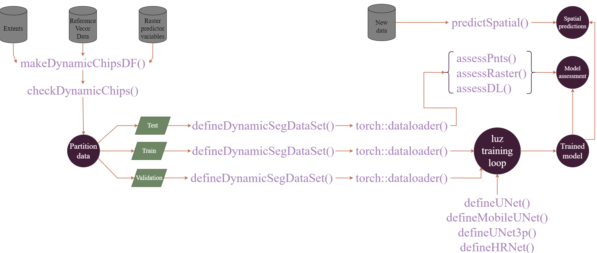
A more recent build of geodl implements an alternative workflow that does not require that predictor variables and associated raster masks be converted into image chips prior to the training or validation process. This workflow is conceptualized in Figure 15.2. The user can specify how to generate image chips and associated masks from processing extents, reference vector geospatial data, and raster-based predictor variables. This DataSet subclass is implemented by the defineDynamicSegDataSet() function and requires first defining a data frame and validating it using the makeDynamicChipsSF() and checkDynamicChips() functions, respectively. This generated data frame contains all the information required to dynamically generate chips using defineDynamicSegDataset().
Although using dynamic chips can slow down the training process, it alleviates the need to generate the chips and associated raster masks beforehand and save them to disk, which can help minimize the disk space required to build the model. The user generally has more control when generating the chips and saving them to disk, or when using the first workflow conceptualized above. However, this second workflow may be more practical in many circumstances.
15.3 Data Preparation
In this section, our goal is to describe the workflow used to prepare data to train and assess DL semantic segmentation models using geodl. Other than geodl, we load the tidyverse, terra, sf, tmap, and tmaptools, and gt. We also define the path to our working directory and the folder where we wish to save output.
fldPth <- "gslrData/chpt15/data/"
outPth <- "gslrData/chpt15/output/"
15.3.1 Raster Masks
For our demonstration, we make use of a subset of an image from the landcover.ai dataset. We also need vector data representing the extent of interest, building footprints, and a wall-to-wall land cover classification. We first display the input image and vector data. The image extent is irregular shaped; however, this is not an issue when using geodl. For the land cover data, all areas in the extent are labeled to one of the following classes: “Background”, “Building”, “Woodland”, “Water”, or “Road.”
plotRGB(img, stretch="lin")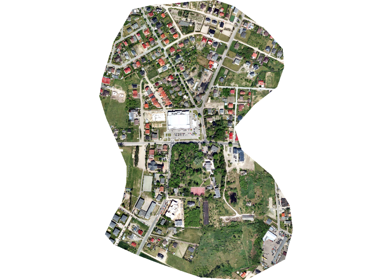
tm_shape(ext)+
  tm_borders(col="red", lwd=2)+
  tm_shape(buildings)+
  tm_polygons(fill="gray")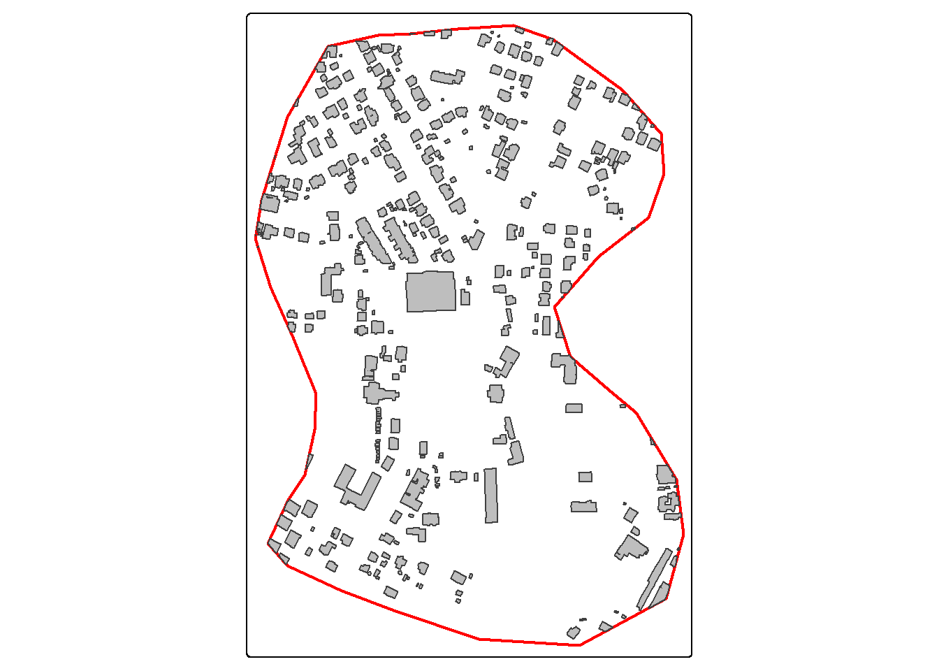
tm_shape(ext)+
  tm_borders(col="red", lwd=2)+
  tm_shape(lc)+
  tm_polygons(fill="gridcode",
              fill.scale = tm_scale_categorical(labels = c("Background",
                                                           "Building",
                                                           "Woodland",
                                                           "Water",
                                                           "Road"
                                                           ),
                                             values = c("gray60",
                                                         "red",
                                                         "green",
                                                         "blue",
                                                         "black")),
            fill.legend = tm_legend("Land Cover"))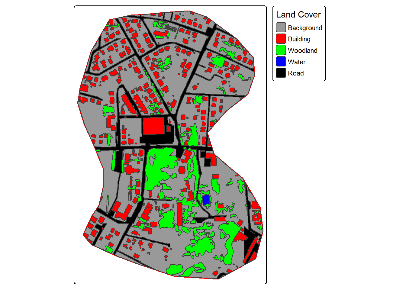
The makeMasks() function is used to convert polygon vector data to categorical raster data. The function requires providing an input image, input polygon vector features, and an attribute column of numeric codes that differentiate each class. A value can also be specified for the background class, or areas occurring outside the reference polygons. For the binary classification of buildings, the “gridcode” column holds a value of 1 for all building features. We are specifying to use a value of 0 for the background class. As a result, the resulting categorical raster will contain values of 0 and 1.
The crop option specifies whether or not the mask should be cropped to a defined extent. In this case, we are cropping the generated raster grid. The mode can be either "Both" or "Mask". When using "Both", a copy of the image is produced alongside of the mask. This is helpful if you want to crop the image relative to an extent and so that the image and mask align perfectly and have the same number of rows and columns of cells.
Once the mask and image are generated, they are read into R as spatRaster objects, and the binary mask is displayed with tmap.
tm_shape(mskB)+
  tm_raster(col.scale = tm_scale_categorical(labels = c("Background",
                                                        "Building"),
                                             values = c("gray60",
                                                         "red")),
            col.legend = tm_legend("Land Cover"))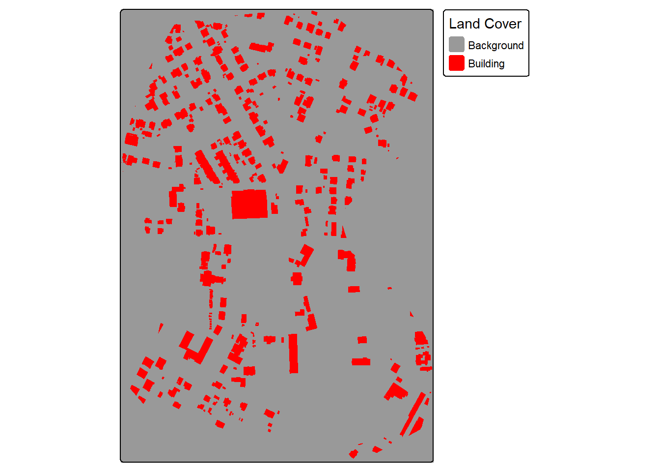
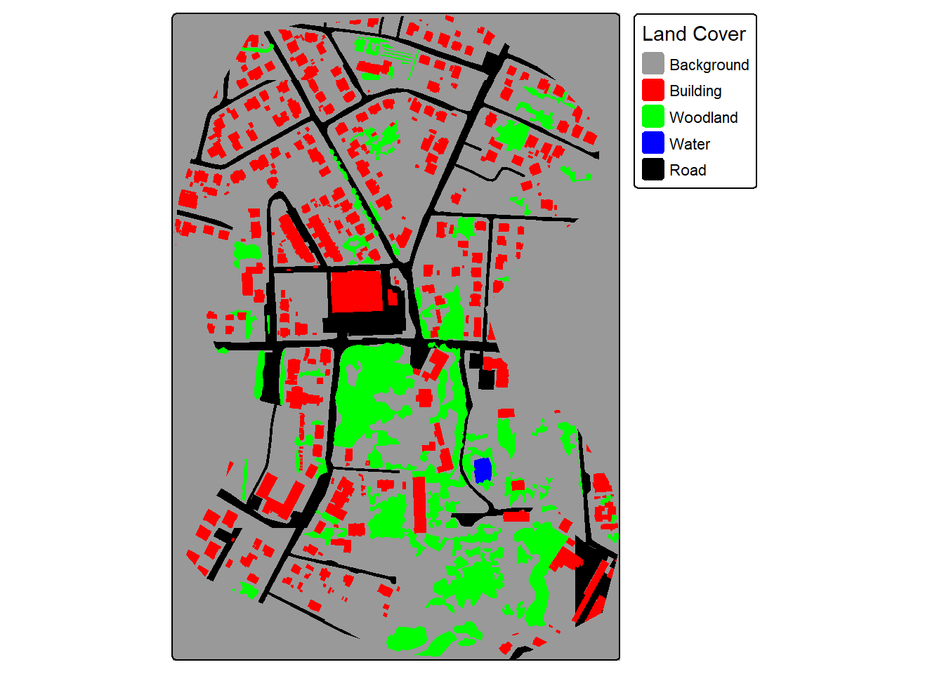
In the second example, we generated masks for the multiclass land cover problem. The setup is the same except now we only create the mask as opposed to the mask and a copy of the image. The “gridcode” column holds values from 0 to 4 representing the five classes being differentiated. The background value of 0 is not used in this case since the polygons completely fill the mapped extent.
15.3.2 Make Chips
Once raster masks are generated that align with the raster-based predictor variables, they can be broken into chips of a defined size using the makeChips() or makeChipsMultiClass() function. makeChips() should be used when there are only two codes, 0 and 1, while makeChipsMultiClass() should be used when there are more than two classes differentiated.
For the building example, we use makeChips(). This function requires specifying the input predictor variables and mask raster grids. The generated chips are saved to a directory indicated by the outDir parameter. Inside this directory, the function will generate “images” and “masks” sub-directories. The size argument specifies the size of each chip, in this case 512x512 cells. The stride_x and stride_y parameters specify how far the moving window moves in the x and y directions as the chips are generated. Since 512 is used, there will be no overlap between adjacent chips. If strides smaller than the chip size are used, overlapping chips are generated.
For a binary classification, three options are available for mode. "All" indicates that all chips are produced including those that contain no cells mapped to the positive case. In contrast, "Positive" indicates that only chips that have at least one cell mapped to the positive case are generated. Lastly, "Divided" indicates that all chips are generated; however, chips that contain only background cells are saved to a separate “Background” directory while those that contain at least one cell mapped to the positive case are saved to the “Positive” directory. Here, we only generating chips with positive-case cells included. You can also save chips to a folder that already exists and contains chips generated from other predictor variable/mask pairs using useExistingDir=TRUE.
If you want to generate chips from multiple datasets, after generating chips from the first datasets, subsequent data can be processed with results saved to the same directory using useExistingDir=FALSE.
For a multiclass problem and when using the makeChipsMultiClass() function, the key differences is that there is no mode argument since there are no background-only samples.
dir.create(str_glue("{outPth}lcChips/"))

makeChipsMultiClass(image = str_glue("{outPth}imgOut.tif"),
                    mask = str_glue("{outPth}lcMskOut.tif"),
                    n_channels = 3,
                    size = 512,
                    stride_x = 512,
                    stride_y = 512,
                    outDir = str_glue("{outPth}lcChips/"),
                    useExistingDir=FALSE)
15.3.3 Make Chips Data Frame
Once chips are created and saved in a specified directory using makeChips() or makeChipsMultiClass(), they can be listed into a data frame using makeChipsDF(). As with makeChips(), for a binary classification, the same three modes are available. For a multiclass classification, you should use mode = "All". For both the binary and multiclass problem types, the generated “chpN” column provides the name of the chip while the “chpPth” and “mskPth” columns list the paths to the images and masks, respectively. For a binary classification and when using mode="Divided", a “Division” column is added to indicate whether the chip is a background-only or positive case-containing sample.
bChipsDF <- makeChipsDF(folder = str_glue("{outPth}bChips/"),
                       extension=".tif",
                       mode="Positive",
                       saveCSV=FALSE)

head(bChipsDF) |>
gt()| chpN | chpPth | mskPth |
|---|---|---|
| imgOut_1025_1025.tif | images/imgOut_1025_1025.tif | masks/imgOut_1025_1025.tif |
| imgOut_1025_1537.tif | images/imgOut_1025_1537.tif | masks/imgOut_1025_1537.tif |
| imgOut_1025_2049.tif | images/imgOut_1025_2049.tif | masks/imgOut_1025_2049.tif |
| imgOut_1025_2561.tif | images/imgOut_1025_2561.tif | masks/imgOut_1025_2561.tif |
| imgOut_1025_513.tif | images/imgOut_1025_513.tif | masks/imgOut_1025_513.tif |
| imgOut_1537_2561.tif | images/imgOut_1537_2561.tif | masks/imgOut_1537_2561.tif |
lcChipsDF <- makeChipsDF(folder = str_glue("{outPth}lcChips/"),
                       extension=".tif",
                       mode="All",
                       saveCSV=FALSE)

head(bChipsDF) |>
gt()| chpN | chpPth | mskPth |
|---|---|---|
| imgOut_1025_1025.tif | images/imgOut_1025_1025.tif | masks/imgOut_1025_1025.tif |
| imgOut_1025_1537.tif | images/imgOut_1025_1537.tif | masks/imgOut_1025_1537.tif |
| imgOut_1025_2049.tif | images/imgOut_1025_2049.tif | masks/imgOut_1025_2049.tif |
| imgOut_1025_2561.tif | images/imgOut_1025_2561.tif | masks/imgOut_1025_2561.tif |
| imgOut_1025_513.tif | images/imgOut_1025_513.tif | masks/imgOut_1025_513.tif |
| imgOut_1537_2561.tif | images/imgOut_1537_2561.tif | masks/imgOut_1537_2561.tif |
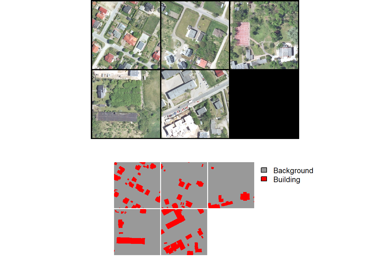
A random subset of chips can be visualized using the viewChips() function. The function requires providing a data frame created with makeChipsDF() and the path to the directory containing the chips. If mode is set to "image", only the images are shown. If mode is set to "mask", only the masks are displayed. Lastly, "both" indicates to show both the images and the masks. The user must also specify the integer or code assigned to each class (cCodes), name of each class (cNames), and color to use to display each class (cColors). If makeChips() is used with mode="Divided", the user can choose to only display chips containing positive case cells using justPositive=TRUE.
We generally recommend visualizing the chips to make sure that the data are being generated as expected. Below, we visualize chips for both the binary and multiclass problems.
viewChips(chpDF=bChipsDF,
          folder=str_glue("{outPth}bChips/"),
          nSamps = 10,
          mode = "both",
          justPositive = FALSE,
          cCnt = 5,
          rCnt = 2,
          r = 1,
          g = 2,
          b = 3,
          rescale = FALSE,
          rescaleVal = 1,
          cCodes = c(0,1),
          cNames= c("Background", "Buildings"),
          cColors= c("gray", "red"),
          useSeed = TRUE,
          seed = 42)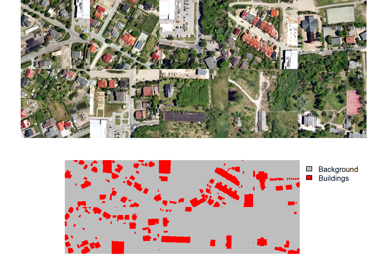
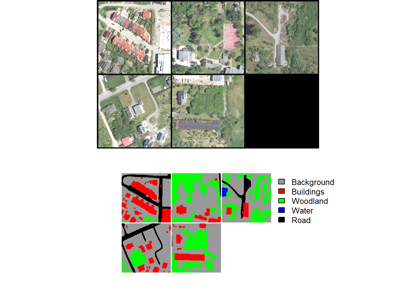
viewChips(chpDF=lcChipsDF,
          folder=str_glue("{outPth}lcChips/"),
          nSamps = 10,
          mode = "both",
          justPositive = FALSE,
          cCnt = 5,
          rCnt = 2,
          r = 1,
          g = 2,
          b = 3,
          rescale = FALSE,
          rescaleVal = 1,
          cCodes = c(0,1,2,3,4),
          cNames= c("Background", "Buildings", "Woodland", "Water", "Road"),
          cColors= c("gray", "red", "green", "blue", "black"),
          useSeed = TRUE,
          seed = 42)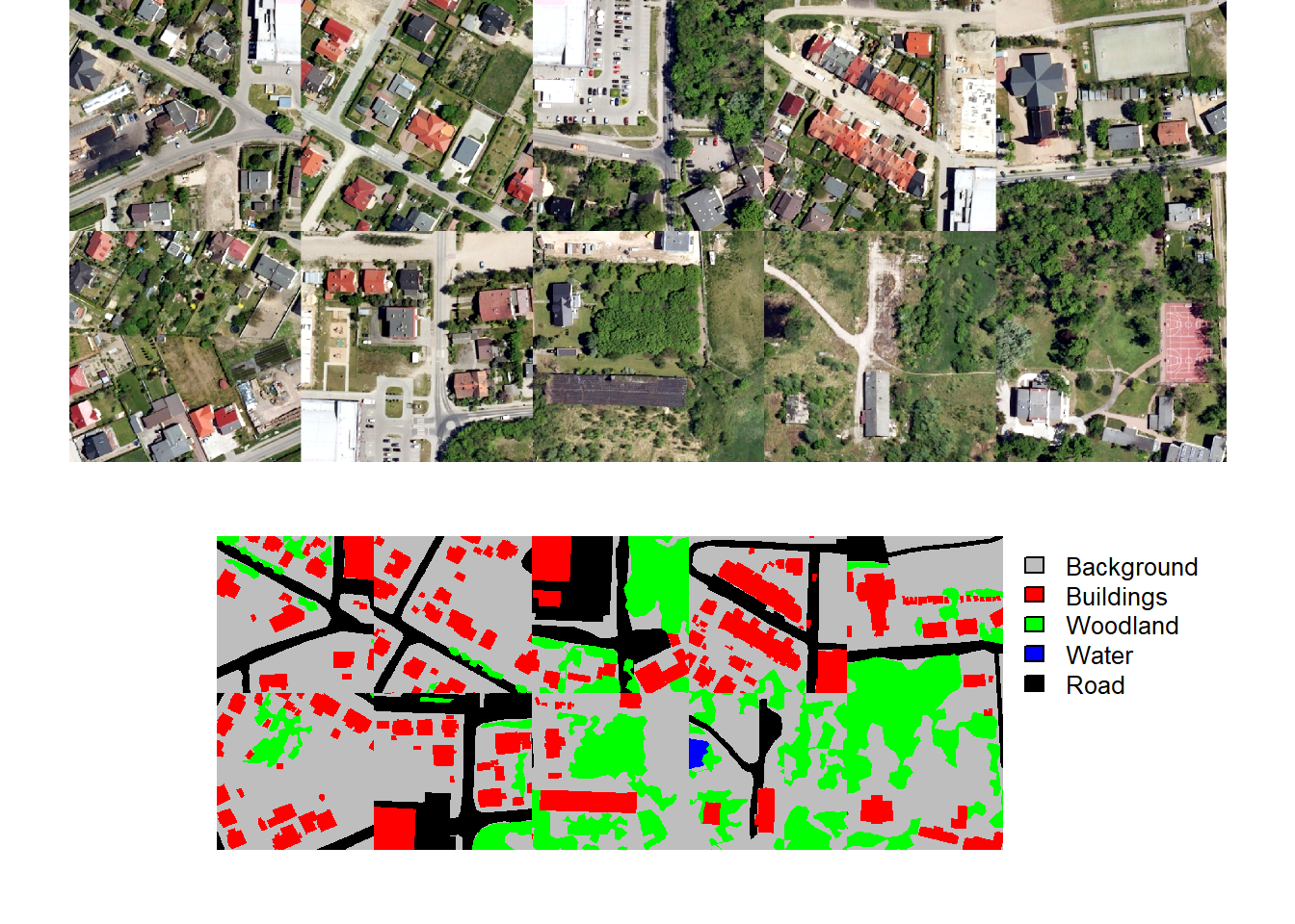
15.3.4 Dataset Subclass
In order to train and validate DL models using torch, input data must be converted into tensors (i.e., multidimensional arrays) with the correct dimensionality and data types. These tensors need to then be provided to the algorithm as mini-batches, since algorithms are trained incrementally on subsets of the available training set. During the training loop, data within each training mini-batch are predicted. These predictions are then compared to the reference labels to calculate a loss (and, optionally, additional assessment metrics). Once the loss is calculated, backpropagation is performed and the model parameters are updated using an optimization algorithm, such as stochastic gradient descent (SGD), RMSProp, or Adam.
In the torch environment, how a single image chip is processed is defined by a dataset subclass. Specifically, the .getitem() method defines how a single input sample is processed to a tensor. The dataLoader is responsible for using the dataset subclass to generate mini-batches of samples to pass to the algorithm during the training or validation processes.
Datasets and dataloaders are used for preparing training, validation, and testing datasets. As a result, they are an important component of the torch workflow. geodl provides the defineSegDataSet() function for processing input data. An instantiated dataset generated with this function can then be passed to torch’s default dataloader class.
The defineSegDataSet() function from geodl instantiates a subclass of torch::dataset() for geospatial semantic segmentation. This function is specifically designed to load data generated using the makeChips() or makeChipsMultiClass() function. It accepts a data frame created with the makeChipsDF() function.
It can also define random augmentations to combat overfitting. Note that horizontal and vertical flips and rotations will impact the alignment of the image chip and associated mask. As a result, the same augmentation will be applied to both the image and the mask to maintain alignment. Changes in brightness, contrast, gamma, hue, and saturation are not applied to the masks since alignment is not impacted by these transformations. Predictor variables are generated with three dimensions (channel/variable, width, height) regardless of the number of channels/variables. Masks are generated as three-dimensional tensors (class index, width, height).
Once the chips have been listed into a data frame and described, a dataset can be defined using defineSegDataSet(). This function has many parameters, many of which relate to data augmentations. Here is a description of the parameters:
chpDF: Data frame of image chip and mask paths created usingmakeChipsDF().folder: Full path or path relative to the working directory to the folder containing the image chips and associated masks. You must include the final forward slash in the path (e.g., “C:/data/chips/”).normalize:TRUEorFALSE. Whether to apply normalization. IfFALSE,bMnsandbSDsare ignored. Default isFALSE. IfTRUE, you must providebMnsandbSDs.rescaleFactor: A re-scaling factor to re-scale the bands to 0 to 1. For example, this could be set to 255 to re-scale 8-bit data. Default is 1 or no re-scaling.mskRescale: Can be used to re-scale binary masks that are not scaled from 0 to 1. For example, if masks are scaled from 0 and 255, you can divide by 255 to obtain a 0 to 1 scale. Default is 1 or no rescaling.-
mskAdd: Value to add to mask class numeric codes. For example, if class indices start are 0, 1 can be added so that indices start at 1. Default is 0 (return original class codes).Note that several other functions in geodl have a
zeroStartparameter. If class codes start at 0, this parameter should be provided an argument ofTRUE. If they start at 1, this parameter should be provided an argument ofFALSE. The importance of this arises from the use of one-hot encoding internally, which requires that class indices start at 1. The key need for this is that R begins indexing at 1 as opposed to 0, which is the case for Python. bands: Vector of bands to include. The default is to only include the first three bands. If you want to use a different subset of bands, you must provide a vector of band indices here to override the default.bMns: Vector of band means. Length should be the same as the number of bands. Normalization is applied before any re-scaling within the function.bSDs: Vector of band standard deviations. Length should be the same as the number of bands. Normalization is applied before any re-scaling.doAugs:TRUEorFALSE. Whether or not to apply data augmentations to combat overfitting. IfFALSE, all augmentation parameters are ignored. Data augmentations are generally only applied to the training set. Default isFALSE.maxAugs: 0 to 7. Maximum number of random augmentations to apply. Default is 0 or no augmentations. Must be changed if augmentations are desired.probVFlip: 0 to 1. Probability of applying vertical flips. Default is 0 or no augmentations. Must be changed if augmentations are desired.probHFlip: 0 to 1. Probability of applying horizontal flips. Default is 0 or no augmentations. Must be changed if augmentations are desired.probRotation: 0 to 1. Probability of applying a rotation by 90-, 180-, or 270-degrees.probBrightness: 0 to 1. Probability of applying brightness augmentation. Default is 0 or no augmentations. Must be changed if augmentations are desired.probContrast: 0 to 1. Probability of applying contrast augmentations. Default is 0 or no augmentations. Must be changed if augmentations are desired.probGamma: 0 to 1. Probability of applying gamma augmentations. Default is 0 or no augmentations. Must be changed if augmentations are desired.probHue: 0 to 1. Probability of applying hue augmentations. Default is 0 or no augmentations. Must be changed if augmentations are desired.probSaturation: 0 to 1. Probability of applying saturation augmentations. Default is 0 or no augmentations. Must be changed if augmentations are desired.brightFactor: Vector of smallest and largest brightness adjustment factors. Random value will be selected between these extremes. The default is 0.8 to 1.2. Can be any non-negative number. For example, 0 gives a black image, 1 gives the original image, and 2 increases the brightness by a factor of 2.contrastFactor: Vector of smallest and largest contrast adjustment factors. Random value will be selected between these extremes. The default is 0.8 to 1.2. Can be any non-negative number. For example, 0 gives a solid gray image, 1 gives the original image, and 2 increases the contrast by a factor of 2.gammaFactor: Vector of smallest and largest gamma values and gain value for a total of three values. Random value will be selected between these extremes. The default gamma value range is 0.8 to 1.2 and the default gain is 1. The gain is not randomly altered, only the gamma. Non-negative real number. A gamma larger than 1 makes the shadows darker while a gamma smaller than 1 makes dark regions lighter.hueFactor: Vector of smallest and largest hue adjustment factors. Random value will be selected between these extremes. The default is -0.2 to 0.2. Should be in range -0.5 to 0.5. 0.5 and -0.5 give complete reversal of hue channel in HSV space in the positive and negative direction, respectively. 0 means no shift. Therefore, both -0.5 and 0.5 will give an image with complementary colors while 0 gives the original image.saturationFactor: Vector of smallest and largest saturation adjustment factors. Random value will be selected between these extremes. The default is 0.8 to 1.2. For example, 0 will give a black-and-white image, 1 will give the original image, and 2 will enhance the saturation by a factor of 2.
In our example, we are re-scaling the data by a factor of 255. This is because the data are currently represented as 8-bit integer values as opposed to 32-bit float values scaled from 0 to 1. We add 1 to the mask codes to obtain values from 1 to 5 as opposed to 0 to 4.
Augmentations are also being performed. A maximum of 3 augmentations will be applied per chip. Vertical flips, horizontal flips, rotation, brightness changes, and saturation changes will be considered. The flips and rotation have a 30% probability of being applied while the brightness and saturation changes have a 10% chance of being applied. We often struggle with determining the appropriate amount of data augmentations to apply. We tend to conservatively apply augmentations; however, others may disagree.
Not all augmentations are appropriate for all data types. For example, saturation and hue adjustments are only applicable to RGB data.
bDS <- defineSegDataSet(chpDF= bChipsDF,
                        folder=str_glue("{outPth}bChips/"),
                        normalize = FALSE,
                        rescaleFactor = 255,
                        mskRescale = 1,
                        mskAdd = 1,
                        bands = c(1, 2, 3),
                        bMns = 1,
                        bSDs = 1,
                        doAugs = TRUE,
                        maxAugs = 3,
                        probVFlip = .3,
                        probHFlip = .3,
                        probRotation = .3,
                        probBrightness = .1,
                        probContrast = .1,
                        probGamma = 0,
                        probHue = 0,
                        probSaturation = .2,
                        brightFactor = c(0.8, 1.2),
                        contrastFactor = c(0.8, 1.2),
                        gammaFactor = c(0.8, 1.2, 1),
                        hueFactor = c(-0.2, 0.2),
                        saturationFactor = c(0.8, 1.2)
)
lcDS <- defineSegDataSet(chpDF= lcChipsDF,
folder=str_glue("{outPth}lcChips/"),
normalize = FALSE,
rescaleFactor = 255,
mskRescale = 1,
mskAdd = 1,
bands = c(1, 2, 3),
bMns = 1,
bSDs = 1,
doAugs = TRUE,
maxAugs = 3,
probVFlip = .3,
probHFlip = .3,
probBrightness = .1,
probContrast = .1,
probGamma = 0,
probHue = 0,
probRotation = .3,
probSaturation = .2,
brightFactor = c(0.8, 1.2),
contrastFactor = c(0.8, 1.2),
gammaFactor = c(0.8, 1.2, 1),
hueFactor = c(-0.2, 0.2),
saturationFactor = c(0.8, 1.2)
)15.3.5 Dataloaders
Once datasets are defined, the base-torch dataloader() function is used to instantiate a dataloader. We use a mini-batch size of 5, shuffle the chips, and drop the last mini-batch. The last mini-batch is dropped because it may be incomplete if the number of available chips is not divisible by the mini-batch size. Calling length() on the generated torch dataloader objects yields the number of mini-batches. Since our example data only include 12 chips and we are using a mini-batch size of 5, only two complete mini-batches can be generated.
bDL <- torch::dataloader(bDS,
                         batch_size=5,
                         shuffle=TRUE,
                         drop_last = TRUE)

lcDL <- torch::dataloader(lcDS,
                          batch_size=5,
                          shuffle=TRUE,
drop_last = TRUE)15.3.6 Checks
geodl provides several functions for checking mini-batches. The viewBatch() function plots a mini-batch of predictor variables and associated masks while the describeBatch() function provides summary information including the number of samples in the mini-batch, the data type of the predictor variables and mask tensors, the shape of the predictor variables and mask mini-batches, predictor variable means and standard deviations, count of cells mapped to each class in the mini-batch, and the minimum and maximum class codes.
Again, it is a good idea to inspect your data prior to training a model. Since the training process can be time consuming, it is best to catch issues prior to starting the training loop.
viewBatch(dataLoader=bDL,
          nCols = 3,
          r = 1,
          g = 2,
          b = 3,
          cCodes = c(1,2),
          cNames=c("Background", "Building"),
          cColors=c("gray60", "red")
)
describeBatch(bDL,
              zeroStart=FALSE)
$batchSize
[1] 5
$imageDataType
[1] "Float"
$maskDataType
[1] "Long"
$imageShape
[1] "5" "3" "512" "512"
$maskShape
[1] "5" "1" "512" "512"
$bndMns
[1] 0.5240634 0.5238758 0.4437808
$bandSDs
[1] 0.1785223 0.1581957 0.1671060
$maskCount
[1] 1098003 212717
$minIndex
[1] 1
$maxIndex
[1] 2viewBatch(lcDL,
nCols = 3,
r = 1,
g = 2,
b = 3,
cCodes=c(1,2,3,4,5),
cNames=c("Background", "Buildings", "Woodland", "Water", "Road"),
cColors=c("gray60", "red", "green", "blue", "black")
)
describeBatch(lcDL,
              zeroStart=FALSE)
$batchSize
[1] 5
$imageDataType
[1] "Float"
$maskDataType
[1] "Long"
$imageShape
[1] "5" "3" "512" "512"
$maskShape
[1] "5" "1" "512" "512"
$bndMns
[1] 0.5248655 0.5249394 0.4446734
$bandSDs
[1] 0.1691765 0.1497183 0.1567565
$maskCount
[1] 686305 165271 258398 4833 195913
$minIndex
[1] 1
$maxIndex
[1] 515.3.7 Dynamic Chips
As noted above, geodl provides an alternative workflow where chips do not need to be generated beforehand. Instead, they are generated dynamically during the training or validation process as needed. This process is conceptualized in Figure 15.2 above. Note that the example data used in this section were not provided since they are large. However, if you want to execute the code, these data can be downloaded from figshare.
The problem being explored is to extract valley fill faces resulting from surface coal mining reclamation using LSP predictor variables. All valley fill faces within three extents have been mapped. We read in the mapped valley fill faces and the extent of the three study areas. This workflow requires that the input polygon vector files contain both “code” and “class” attributes. The “code” field provides a unique numeric code for each class. In this case, we use a code of 1 since there is only one class being differentiated. Since the data do not include a “class” attribute, we generate this attribute, populate it with “vfill”, and save a copy of the file to disk with st_write().
fldPth2 <- "D:/22318522/vfillDL/vfillDL/"ky1Ext <- st_read(str_glue("{fldPth2}extents/testingKY1.shp"), quiet=TRUE)
ky2Ext <- st_read(str_glue("{fldPth2}extents/testingKY2.shp"), quiet=TRUE)
va1Ext <- st_read(str_glue("{fldPth2}extents/testingVA1.shp"), quiet=TRUE)
ky1V <- st_read(str_glue("{fldPth2}vectors/testingKY1.shp"), quiet=TRUE) |>
mutate(class = "vfill") |>
st_write(str_glue("{fldPth2}vectors/testingKY1b.shp"),
append=TRUE)
ky2V <- st_read(str_glue("{fldPth2}vectors/testingKY2.shp"), quiet=TRUE) |>
mutate(class = "vfill") |>
st_write(str_glue("{fldPth2}vectors/testingKY2b.shp"),
append=TRUE)
va1V <- st_read(str_glue("{fldPth2}vectors/testingVA1.shp"), quiet=TRUE) |>
mutate(class = "vfill") |>
st_write(str_glue("{fldPth2}vectors/testingVA1b.shp"),
append=TRUE)Next, we plot the three extents, which occur in eastern Kentucky and southwestern Virginia, USA.
allExtents <- bind_rows(ky1Ext, ky2Ext, va1Ext)
allFeatures <- bind_rows(ky1V, ky2V, va1V)
allFeaturesPnts <- st_centroid(allFeatures)

osm <- read_osm(st_bbox(st_buffer(allExtents, 3000)))

tm_shape(osm)+
  tm_rgb()+
  tm_shape(allExtents)+
  tm_borders(col="black", lwd=2)+
  tm_shape(allFeaturesPnts)+
  tm_bubbles(fill="red", size=.5)+
  tm_compass(position=c("left", "bottom"))+
  tm_scalebar(position=c("left", "bottom"))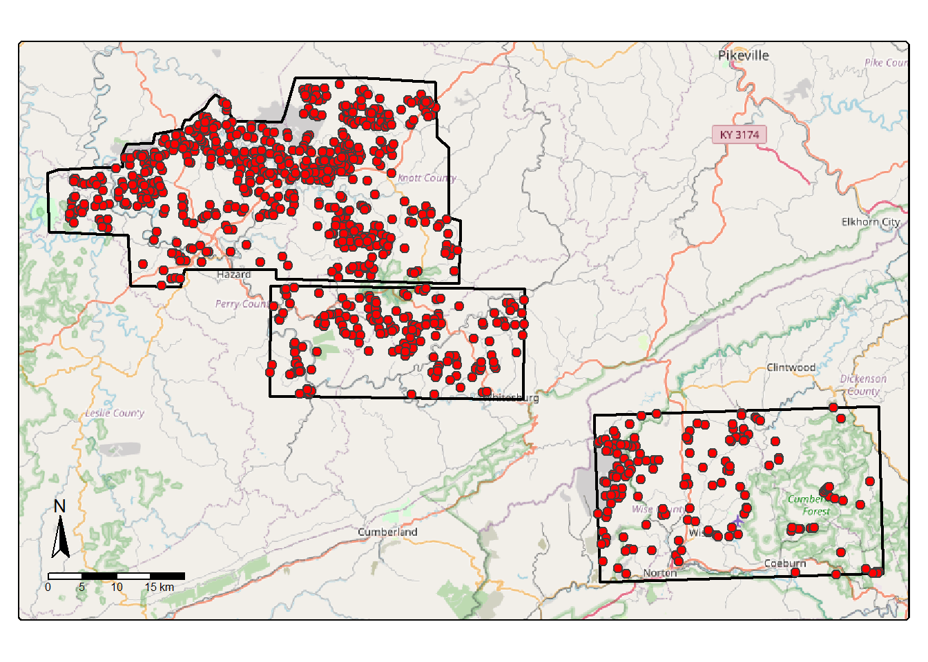
The makeDynamicChipsSF() function is used to create an sf vector object that specifies the center location of each chip to generate. The required inputs include the path to and name of the feature layer and extent vector boundary and the path to and name of the raster predictor variable data. In order to minimize partial or incomplete chips, a crop can be applied to the extent using the extentCrop parameter. We use a crop of 200 m in our example. For binary classification tasks, it is also possible to generate random background chips. In this case, we generate 300 background chips where the center cannot be within 100 meters of a positive-case chip center. In order to make this reproducible, it is possible to set a random seed. Lastly, the order of the chips can be changed via shuffling to potentially reduce spatial autocorrelation.
In our example, we process all three extents separately then merge the result into a single sf object.
ky1DC <- makeDynamicChipsSF(
  featPth = str_glue("{fldPth2}vectors/"),
  featName = "testingKY1b.shp",
  extentPth = str_glue("{fldPth2}extents/"),
  extentName = "testingKY1.shp",
  extentCrop = 200,
  imgPth <- str_glue("{fldPth2}dems/"),
  imgName <- "ky1_dem.tif",
  doBackground = TRUE,
  backgroundCnt = 300,
  backgroundDist = 100,
  useSeed = TRUE,
  seed = 42,
  doShuffle = TRUE
)

ky2DC <- makeDynamicChipsSF(
  featPth = str_glue("{fldPth2}vectors/"),
  featName = "testingKY2b.shp",
  extentPth = str_glue("{fldPth2}extents/"),
  extentName = "testingKY2.shp",
  extentCrop = 200,
  imgPth <- str_glue("{fldPth2}dems/"),
  imgName <- "ky_2_dem.tif",
  doBackground = TRUE,
  backgroundCnt = 300,
  backgroundDist = 100,
  useSeed = TRUE,
  seed = 42,
  doShuffle = TRUE
)

va1DC <- makeDynamicChipsSF(
  featPth = str_glue("{fldPth2}vectors/"),
  featName = "testingVA1b.shp",
  extentPth = str_glue("{fldPth2}extents/"),
  extentName = "testingVA1.shp",
  extentCrop = 200,
  imgPth <- str_glue("{fldPth2}dems/"),
  imgName <- "va1_dem.tif",
  doBackground = TRUE,
  backgroundCnt = 300,
  backgroundDist = 100,
  useSeed = TRUE,
  seed = 42,
  doShuffle = TRUE
)

allDC <- bind_rows(ky1DC, ky2DC, va1DC)
Once the sf objects are generated, the dynamic chips should be checked using the checkDynamicChips() function. This requires generating each chip in memory and calculating summary information. We use the results to remove any chip that is smaller than the desired size, 512x512, and/or that contain NA cells. This results in chips that are of the correct size and do not have any missing data.
allDC <- checkDynamicChips(chipsSF = allDC,
                           chipSize=512,
                           cellSize=2,
                           doJitter=TRUE,
                           jitterSD=15,
                           useSeed=TRUE,
                           seed=42)
allDC <- allDC |> filter(cCntImg == 512 &
rCntImg == 512 &
cCntMsk == 512 &
rCntMsk == 512 &
naCntImg == 0 &
naCntMsk == 0)Similar to the prior workflow, we next instantiate an instance of the torch dataset subclass and a dataloader. The dataset is created using the defineDynamicSegDataSet() function and requires setting a desired chip size. Random noise can also be added to the chip center coordinates if desired. The same normalization, re-scaling, and data augmentation options provided by defineSegDataSet() are available.
allDCDS <- defineDynmamicSegDataSet(chipsSF=allDC,
                        chipSize=512,
                        cellSize=2,
                        doJitter=TRUE,
                        jitterSD=15,
                        useSeed=TRUE,
                        seed=42,
                        normalize = FALSE,
                        rescaleFactor = 1,
                        mskRescale=1,
                        mskAdd=1)
allDL <- torch::dataloader(allDCDS,
batch_size=10,
shuffle=TRUE,
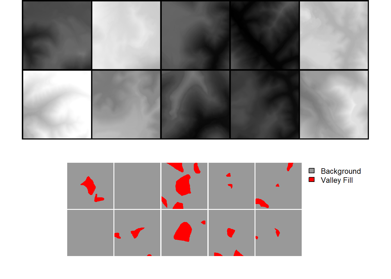
drop_last = TRUE)length(allDL)[1] 243Once the dataloader is defined, results can be visualized with viewBatch(), just as when using the other workflow. If you desire to save the chips or a subset of the chips to disk, this can be accomplished with the saveDynamicChips() function. We demonstrate this in the final code block for a random subset of 20 chips.
viewBatch(dataLoader=allDL,
          nCols = 5,
          r = 1,
          g = 1,
          b = 1,
          cCodes = c(1,2),
          cNames=c("Background", "Valley Fill"),
          cColors=c("gray60", "red")
)
allDCSub <- allDC |> sample_n(20, replace=FALSE)

dir.create(str_glue("{outPth}dynamicChips/"))

saveDynamicChips(chipsSF = allDCSub,
                 chipSize=512,
                 cellSize=1,
                 outDir=str_glue("{outPth}dynamicChips/"),
                 mode = "All",
                 useExistingDir = FALSE,
                 doJitter=FALSE,
                 jitterSD=15,
                 useSeed=TRUE,
                 seed=42)
This workflow is still experimental. However, it may be more convenient for many use cases.
15.4 Models
15.4.1 UNet
As discussed in the prior chapter, UNet was originally introduced in the following paper:
Ronneberger, O., Fischer, P. and Brox, T., 2015. U-net: Convolutional networks for biomedical image segmentation. In Medical image computing and computer-assisted intervention–MICCAI 2015: 18th international conference, Munich, Germany, October 5-9, 2015, proceedings, part III 18 (pp. 234-241). Springer international publishing.
It is an encoder-decoder architecture with a “U” shape. The encoder learns patterns or feature maps at multiple spatial scales and consist of double-convolution blocks as conceptualized in Figure 15.3(a). Each block consists of the following chain of operations where convolutional layers make use of a 3x3 kernel with a stride of 1 and padding of 1 so that the spatial resolution and number of rows and columns of pixels are maintained:
3x3 2D Convolution –> Batch Normalization –> Activation Function –> 3x3 2D Convolution –> Batch Normalization –> Activation function
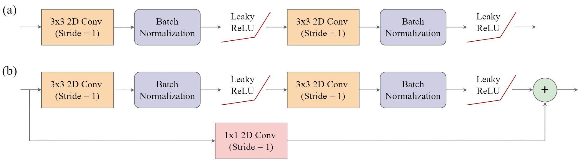
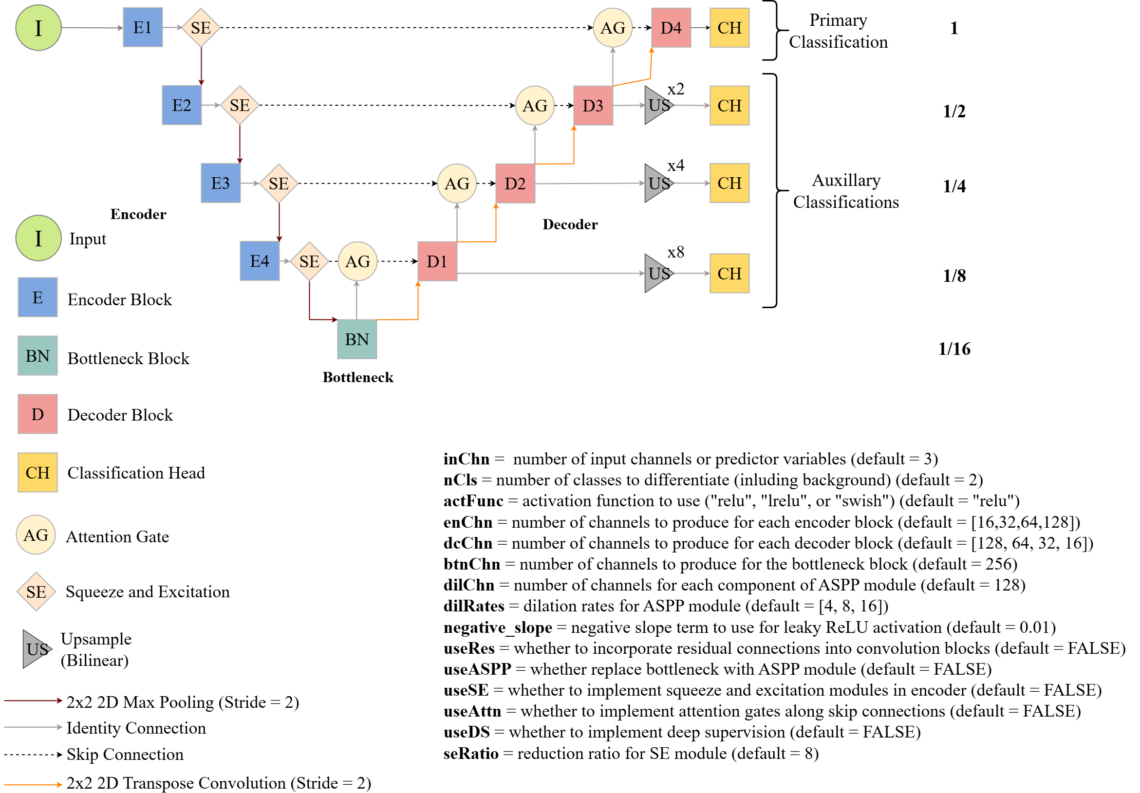
Figure 15.4 conceptualizes the UNet architecture implemented by geodl using the defineUNet() function. The user is able to define the number of input predictor variables (inChn), number of output classes (nCls), number of feature maps generated by each encoder block (enChn), number of feature maps generated by the bottleneck block (btnChn), and number of feature maps generated by each decoder block (dcChn). The user can choose between the following activation functions using the actFunc parameter: rectified linear unit (ReLU) ("relu"), leaky ReLU ("lrelu"), or swish ("swish"). If leaky ReLU is used, the negative_slope parameter defines the negative slope term, which is 0.01 by default. If useRes=TRUE, a residual connection is included within each block, as conceptualized in Figure 15.3(b) above. This can be helpful to combat the vanishing gradient problem. Since the number of output feature maps are different from the number of input feature maps, a 1x1 2D convolution is used to change the number of feature maps along the projection connection.
Please consult the following paper to learn more about the modules and options for geodl’s UNet architecture:
Maxwell, A.E., Farhadpour, S., Das, S. and Yang, Y., 2024. geodl: An R package for geospatial deep learning semantic segmentation using torch and terra. PloS one, 19(12), p.e0315127.
This implementation also supports some additional modifications. Squeeze and excitation modules can be included between the encoder blocks using useSE=TRUE while attention gates can be included along the skip connections using useAttn=TRUE. If squeeze and excitation is used, the seRatio parameter allows the user to define the reduction ratio. The default double-convolution bottleneck block can be replaced with an atrous spatial pyramid (ASPP) module using useASPP=TRUE. If this modification is applied, the dilChn parameters defines the number of channels to generate in each component of the module while the dilRates parameter specifies the dilation rates to use. Lastly, deep supervision can be implemented using doDS=TRUE. If deep supervision is implemented, the model will generate output logits using all stages of the decoder. For all stages other than the final, the output is up-scaled using bilinear interpolation to match that of the input data. The multiple results can be used with the unified focal loss framework.
The following code shows how to instantiate a UNet model using defineUNet() and use it to predict a tensor of random values with the correct shape as a test. The countParams() function from geodl returns the number of trainable parameters included in the model.
unetMod <- defineUNet(inChn = 4,
                      nCls = 7,
                      actFunc = "lrelu",
                      useAttn = TRUE,
                      useSE = TRUE,
                      useRes = TRUE,
                      useASPP = TRUE,
                      useDS = FALSE,
                      enChn = c(16, 32, 64, 128),
                      dcChn = c(128, 64, 32, 16),
                      btnChn = 256,
                      dilRates = c(6, 12, 18),
                      dilChn = c(256, 256, 256, 256),
                      negative_slope = 0.01,
                      seRatio = 8
)$to(device="cuda")
t1 <- torch::torch_rand(c(12,4,256,256))$to(device="cuda")
p1 <- unetMod(t1)p1$shape[1] 12 7 256 256countParams(unetMod, t1)$total_trainable
[1] 2827651
$total_non_trainable
[1] 0
$layer_params
layer trainable non_trainable
1 ag1 883 0
2 ag2 3299 0
3 ag3 12739 0
4 ag4 50051 0
5 btn 1249280 0
6 c4 119 0
7 d1 639872 0
8 d2 160192 0
9 d3 40160 0
10 d4 10096 0
11 dUp1 262912 0
12 dUp2 65920 0
13 dUp3 16576 0
14 dUp4 4192 0
15 e1 3056 0
16 e2 14560 0
17 e3 57792 0
18 e4 230272 0
19 se1 80 0
20 se2 288 0
21 se3 1088 0
22 se4 4224 0
$input_size
[1] 12 4 256 256
$output_size
[1] 12 7 256 25615.4.2 UNet with MobileNetv2 Encoder
The package also implements a version of UNet with a MobileNetv2 encoder (defineMobileUNet()). This implementation was inspired by a Posit blog post by Sigrid Keydana. The MobileNetv2 scene labeling architecture was introduced in the following manuscript and was built to support efficient model training on resource constrained devices. geodl make use of the version of the architecture provided by the torchvision R package.
Sandler, M., Howard, A., Zhu, M., Zhmoginov, A. and Chen, L.C., 2018. Mobilenetv2: Inverted residuals and linear bottlenecks. In Proceedings of the IEEE conference on computer vision and pattern recognition (pp. 4510-4520).
This version contains five encoder blocks, the bottleneck, and five decoder blocks. Components from MobileNetv2 are used for all encoder blocks and the bottleneck block. The layers or stages of MobileNetv2 that are used for each encoder block are noted in Figure 15.5. Max pooling is not implemented between encoder blocks since MobileNetv2 includes downsampling as part of its architecture.
The user is able to use pre-trained ImageNet weights (pretrainedEncoder=TRUE) for the encoder, and the encoder parameters can be updated (freezeEncoder=FALSE) or remain frozen (freezeEnoder=TRUE) during the training process. Similar to the UNet implementation discussed above, the implementation allows for selecting an activation function to use in the decoder blocks (actFunc) and defining the number of output feature maps from each decoder block (dcChn). The user is not able to set the number of outputs for the encoder or bottleneck blocks since this is defined by the MobileNetv2 architecture. Similar to the UNet architecture described above, attention gates can be added along the skip connections (useAttn=TRUE) and deep supervision can be implemented (doDS=TRUE). If deep supervision is implemented, classifications from decoder blocks 2 through 5 are used with upsampling applied to generate output at the original spatial resolution.
If a pre-trained encoder is used and the input data have a number of bands other than three, an average of the loaded weights are used for all layers in the first layer of the architecture. If three inputs are used, the original weights or the averaged weights can be used.

The code below demonstrates how to instantiate an instance of this architecture, use it to predict random data, and obtain a count of trainable parameters.
munetMod <- defineMobileUNet(inChn = 4,
                             nCls = 7,
                             pretrainedEncoder = TRUE,
                             freezeEncoder = FALSE,
                             avgImNetWeights = TRUE,
                             actFunc = "lrelu",
                             useAttn = FALSE,
                             useDS = FALSE,
                             dcChn = c(256, 128, 64, 32, 16),
                             negative_slope = 0.01
)$to(device="cuda")
t1 <- torch::torch_rand(c(12,4,256,256))$to(device="cuda")
p1 <- munetMod(t1)p1$shape[1] 12 7 256 256countParams(munetMod, t1)$total_trainable
[1] 6460095
$total_non_trainable
[1] 0
$layer_params
layer trainable non_trainable
1 base_model 3505160 0
2 c4 119 0
3 d1 1549824 0
4 d2 480000 0
5 d3 124800 0
6 d4 32448 0
7 d5 7584 0
8 dUp1 410560 0
9 dUp2 262912 0
10 dUp3 65920 0
11 dUp4 16576 0
12 dUp5 4192 0
$input_size
[1] 12 4 256 256
$output_size
[1] 12 7 256 25615.4.3 UNet3+
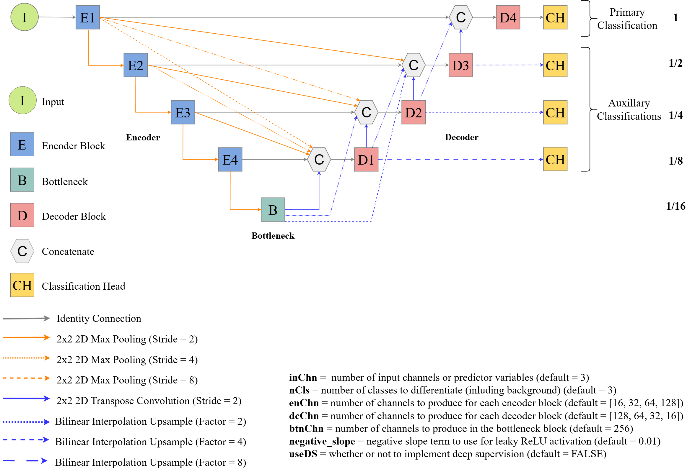
UNet3+ (Figure 15.6) expands upon base UNet by incorporating additional connections and skip connections within the architecture. This requires downsampling with max pooling using varying strides or upsampling using bilinear interpolation using varying factors. This architecture was originally introduced by:
Huang, H., Lin, L., Tong, R., Hu, H., Zhang, Q., Iwamoto, Y., Han, X., Chen, Y.W. and Wu, J., 2020, May. Unet 3+: A full-scale connected unet for medical image segmentation. In ICASSP 2020-2020 IEEE international conference on acoustics, speech and signal processing (ICASSP) (pp. 1055-1059). IEEE.
A modified version of the UNet3+ architecture is implemented within geodl via the defineUNet3p() function. It allows for defining the number of input channels (inChn), number of output classes (nCls), number of feature maps generated by each encoder block (enChn), number of feature maps generated by the bottleneck block (btnChn), and the number of feature maps generated by each decoder block (dcChn). It also allows for selecting the activation function to use throughout the architecture (actFunc) and using deep supervision (doDS=TRUE).
Due to the larger number of input feature maps resulting from the skip connections, this architecture will generally have a larger number of trainable parameters than base UNet and requires more time to train. However, the increased degree of connection and sharing of multi-scale spatial information throughout the architecture may improve the resulting classification.
The code below demonstrates how to instantiate an instance of this architecture, use it to predict random data, and obtain a count of trainable parameters.
unet3pMod <- defineUNet3p(inChn = 4,
                          nCls = 7,
                          useDS = FALSE,
                          enChn = c(16, 32, 64, 128),
                          dcChn = c(128, 64, 32, 16),
                          btnChn = 256,
                          negative_slope = 0.01
)$to(device="cuda")
t1 <- torch::torch_rand(c(12,4,256,256))$to(device="cuda")
p1 <- unet3pMod(t1)p1$shape[1] 12 7 256 256countParams(unet3pMod, t1)$total_trainable
[1] 2745548
$total_non_trainable
[1] 0
$layer_params
layer trainable non_trainable
1 bottleneck 886272 0
2 ch1 903 0
3 ch2 455 0
4 ch3 231 0
5 ch4 119 0
6 decoder1 719616 0
7 decoder1up 262912 0
8 decoder2 322944 0
9 decoder2up 65920 0
10 decoder3 152256 0
11 decoder3up 16576 0
12 decoder4 18528 0
13 decoder4up 4192 0
14 encoder1 2976 0
15 encoder2 14016 0
16 encoder3 55680 0
17 encoder4 221952 0
$input_size
[1] 12 4 256 256
$output_size
[1] 12 7 256 25615.4.4 HRNet
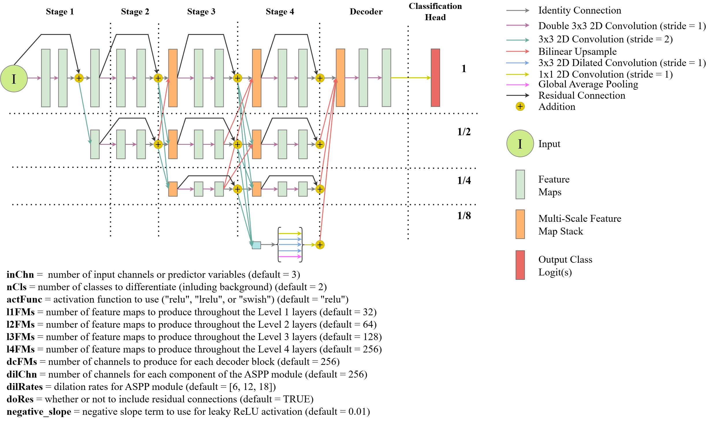
Lastly, geodl also implements a modified version of the HRNet architecture (FIgure 15.7) after:
Wang, J., Sun, K., Cheng, T., Jiang, B., Deng, C., Zhao, Y., Liu, D., Mu, Y., Tan, M., Wang, X. and Liu, W., 2020. Deep high-resolution representation learning for visual recognition. IEEE transactions on pattern analysis and machine intelligence, 43(10), pp.3349-3364.
The key innovation of this architecture is that it maintains high spatial resolution representations of the data, or feature maps, throughout the architecture. Higher resolution data are reduced in size using strides larger than one, and lower spatial resolution feature maps are upsampled using bilinear interpolation. At the beginning of each stage, feature maps are concatenated and shared between layers to make use of the multi-scale information learned by the prior stage of the model.
The key differences between the geodl implementation and the originally proposed implementation includes expanding the decoder component to include more convolutional layers and using an atrous spatial pyramid pooling (ASPP) module at the lowest resolution. The user can define the number of input channels (inChn), number of output classes (nCls), number of feature maps generated by each level in the encoder blocks (lChn), number of feature maps generated by each decoder block (btnChn), and the number of feature maps generated by each component of the ASPP module (dilChn) and associated dilation rates (dilRates). The user can also specify which activation function to use throughout the architecture with the actFunc parameter.
This is the largest of the models made available by geodl; as a result, it may need to be trained with a smaller mini-batch size and/or using smaller image chips. It may be useful when features of interest vary in size, when complex boundary delineation is required, and/or when features of interest are small.
The code below demonstrates how to instantiate an instance of this architecture, use it to predict random data, and obtain a count of trainable parameters.
hrnetMod <- defineHRNet(inChn = 4,
                        nCls = 7,
                        l1FMs = 32,
                        l2FMs = 64,
                        l3FMs = 128,
                        l4FMs = 256,
                        dcFMs = 256,
                        dilChn = c(256, 256, 256, 256),
                        dilRates = c(6, 12, 18),
                        doRes = TRUE,
                        actFunc = "lrelu",
                        negative_slope = 0.01
)$to(device="cuda")
t1 <- torch::torch_rand(c(2,4,256,256))$to(device="cuda")
p1 <- hrnetMod(t1)p1$shape[1] 2 7 256 256countParams(hrnetMod, t1)$total_trainable
[1] 6553319
$total_non_trainable
[1] 0
$layer_params
layer trainable non_trainable
1 ch 1799 0
2 dcBlk 1820416 0
3 s1l1a 10720 0
4 s1l1aDown2 9312 0
5 s1l1b 9312 0
6 s1l2b 18624 0
7 s2l1a 19680 0
8 s2l1aDown2 9312 0
9 s2l1aDown4 9312 0
10 s2l1b 27744 0
11 s2l2a 78272 0
12 s2l2aDown2 37056 0
13 s2l2aUp2 4288 0
14 s2l2b 55488 0
15 s2l3b 110976 0
16 s3l1a 19680 0
17 s3l1aDown2 9312 0
18 s3l1aDown4 9312 0
19 s3l1aDown8 9312 0
20 s3l1b 64608 0
21 s3l2a 78272 0
22 s3l2aDown2 37056 0
23 s3l2aDown4 37056 0
24 s3l2aUp2 4288 0
25 s3l2b 129216 0
26 s3l3a 312192 0
27 s3l3aDown2 147840 0
28 s3l3aUp2 16768 0
29 s3l3aUp4 16768 0
30 s3l3b 258432 0
31 s3l4b 516864 0
32 s4l1a 19680 0
33 s4l2a 78272 0
34 s4l2aUp2 4288 0
35 s4l3a 312192 0
36 s4l3aUp4 16768 0
37 s4l4a 2166528 0
38 s4l4aUp8 66304 0
$input_size
[1] 2 4 256 256
$output_size
[1] 2 7 256 25615.5 Unified Focal Loss
geodl provides a modified version of the unified focal loss proposed in the following study:
Yeung, M., Sala, E., Schönlieb, C.B. and Rundo, L., 2022. Unified focal loss: Generalising dice and cross entropy-based losses to handle class imbalanced medical image segmentation. Computerized Medical Imaging and Graphics, 95, p.102026.
Table 15.1 describes the loss parameterization. The geodl implementation is different from the originally proposed implementation because it does not implement symmetric and asymmetric forms. Instead, it allows the user to define class weights for both the distribution- and region-based loss components.
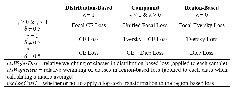
The lambda parameter controls the relative weighting between the distribution- and region-based losses. When lambda=1, only the distribution-based loss is used. When lambda=0, only the region-based loss is used. Values between 0 and 1 yield a loss metric that incorporates both the distribution- and region-based loss components. A lambda of 0.5 yield equal weighting, values larger than 0.5 put more weight on the distribution-based loss, and values lower than 0.5 put more weighting on the region-based loss.
The gamma parameter controls the weight applied to difficult-to-predict samples, defined as samples or classes with low predicted re-scaled logits relative to their correct class. For the distribution-based loss, focal corrections are implemented sample-by-sample. For the region-based loss, corrections are implemented class-by-class during macro-averaging. gamma must be larger than 0 and less than or equal to 1. When gamma=1, no focal correction is applied. Lower values result in a larger focal correction.
The delta parameter controls the relative weights of false negative (FN) and false positive (FP) errors and should be between 0 and 1. A delta of 0.5 places equal weight on FN and FP errors. Values larger than 0.5 place more weight on FN in comparison to FP errors while values smaller than 0.5 place more weight on FP samples in comparison to FN samples.
The clsWghtDist parameter controls the relative weights of classes in the distribution-based loss and is applied sample-by-sample. The clsWghtReg parameter controls the relative weights of classes in the region-based loss and are applied to each class when calculating a macro average. By default, all classes are weighted equally. If you want to implement class weights, you must provide a vector of class weights equal in length to the number of classes being differentiated.
Lastly, the useLogCosH parameter determines whether or not to apply a log cosh transformation to the region-based loss. If it is set to TRUE, this transformation is applied.
Using different parameterizations, users can define a variety of loss metrics including cross entropy (CE) loss, weighted CE loss, focal CE loss, focal weighted CE loss, Dice loss, focal Dice loss, Tversky loss, and focal Tversky loss.
15.5.1 Loss Examples
We will now demonstrate how different loss metrics can be obtained using different parameterizations. We first load in example data using the rast() function from terra representing class reference numeric codes (refC) and predicted class logits (predL).
tm_shape(refC)+
    tm_raster(col.scale = tm_scale_categorical(labels = c("Background",
                                                           "Building",
                                                           "Woodland",
                                                           "Water",
                                                           "Road"
                                                           ),
                                             values = c("gray60",
                                                         "red",
                                                         "green",
                                                         "blue",
                                                         "black")),
            col.legend = tm_legend("Land Cover"))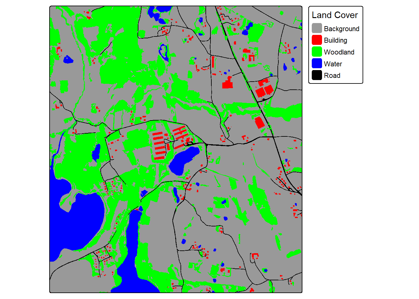
plot(predL)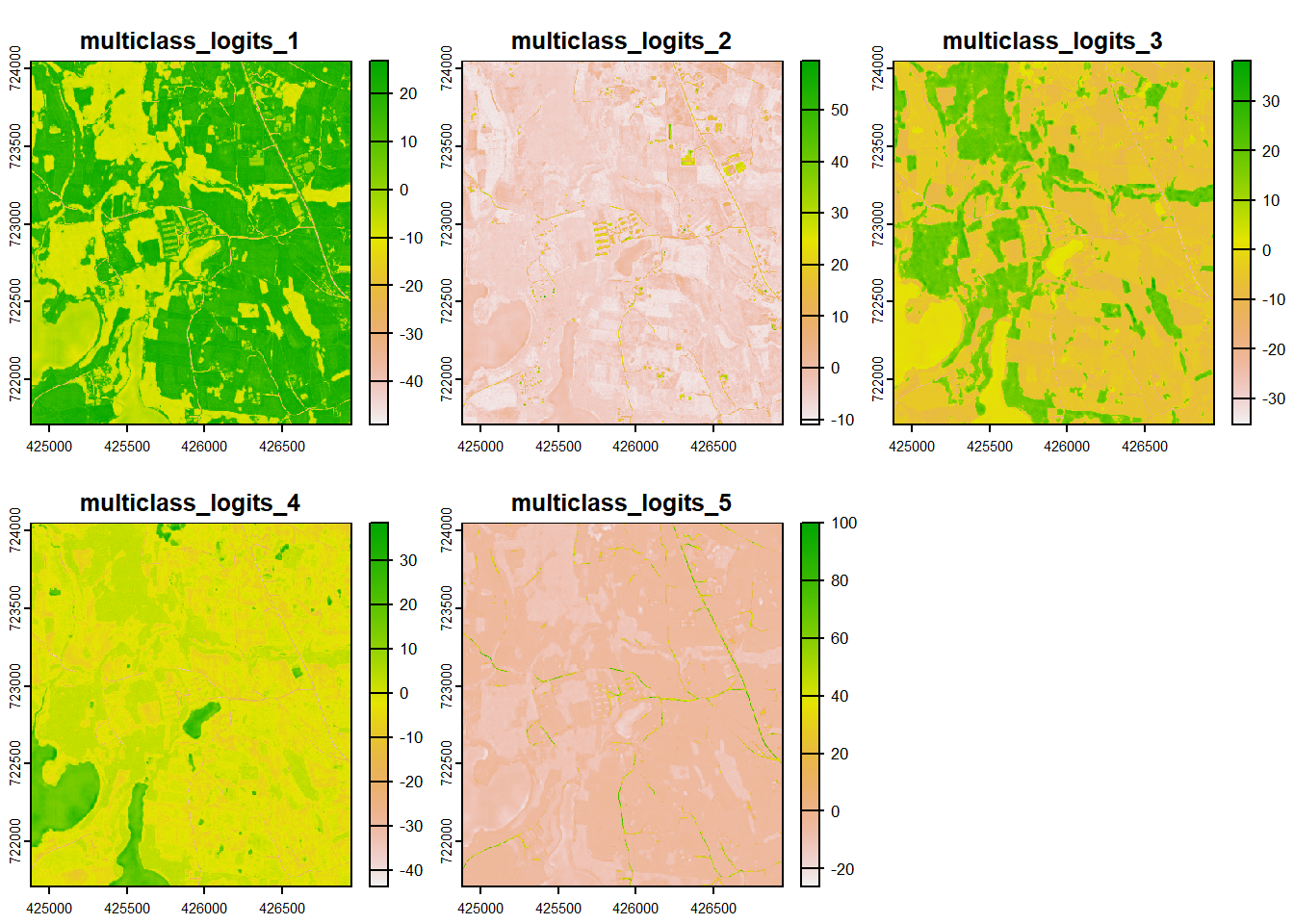
The spatRaster objects are then converted to torch tensors with the correct shape and data type. We simulate a mini-batch of two samples by concatenating two copies of the tensors.
predL <- terra::as.array(predL)
refC <- terra::as.array(refC)

target <- torch::torch_tensor(refC, dtype=torch::torch_long(), device="cuda")
pred <- torch::torch_tensor(predL, dtype=torch::torch_float32(), device="cuda")
target <- target$permute(c(3,1,2))
pred <- pred$permute(c(3,1,2))

target <- target$unsqueeze(1)
pred <- pred$unsqueeze(1)

target <- torch::torch_cat(list(target, target), dim=1)
pred <- torch::torch_cat(list(pred, pred), dim=1)
15.5.1.1 Example 1: Dice Loss
The Dice loss is obtained by setting the lambda parameter to 0, the gamma parameter to 1, and the delta parameter to 0.5. This results in only the region-based loss being considered, no focal correction being applied, and equal weighting between FN and FP errors.
myDiceLoss <- defineUnifiedFocalLoss(nCls=5,
                                 lambda=0, #Only use region-based loss
                                 gamma= 1,
                                 delta= 0.5, #Equal weights for FP and FN
                                 smooth = 1e-8,
                                 zeroStart=TRUE,
                                 clsWghtsDist=1,
                                 clsWghtsReg=1,
                                 useLogCosH =FALSE,
                                 device="cuda")
myDiceLoss(pred=pred,
           target=target)
torch_tensor
0.17861
[ CUDAFloatType{} ]15.5.1.2 Example 2: Tversky Loss
The Tversky Loss can be obtained using the same settings as those used for the Dice loss except that the delta parameter must be set to a value other than 0.5 so that different weights are applied to FN and FP errors. In the example, we use a weighting of 0.6, which places more weight on FN errors relative to FP errors. Setting gamma to a value lower than 1 results in a focal Tversky loss.
We must regenerate the tensors so that the computational graphs are re-initialized.
target <- torch::torch_tensor(refC, dtype=torch::torch_long(), device="cuda")
pred <- torch::torch_tensor(predL, dtype=torch::torch_float32(), device="cuda")
target <- target$permute(c(3,1,2))
pred <- pred$permute(c(3,1,2))

target <- target$unsqueeze(1)
pred <- pred$unsqueeze(1)
target <- torch::torch_cat(list(target, target), dim=1)
pred <- torch::torch_cat(list(pred, pred), dim=1)

myTverskyLoss <- defineUnifiedFocalLoss(nCls=5,
                                        lambda=0, #Only use region-based loss
                                        gamma= 1,
                                        delta= 0.6, #FN weighted higher than FP
                                        smooth = 1e-8,
                                        zeroStart=TRUE,
                                        clsWghtsDist=1,
                                        clsWghtsReg=1,
                                        useLogCosH =FALSE,
                                        device="cuda")

myTverskyLoss(pred=pred,
              target=target)
torch_tensor
0.177986
[ CUDAFloatType{} ]15.5.1.3 Example 3: Cross Entropy (CE) Loss
The cross entropy (CE) loss is obtained by setting lambda to 1, so that only the distribution-based loss is considered, and setting gamma to 1, so that no focal correction is applied. Setting gamma to a value lower than 1 results in a focal CE loss.
target <- torch::torch_tensor(refC, dtype=torch::torch_long(), device="cuda")
pred <- torch::torch_tensor(predL, dtype=torch::torch_float32(), device="cuda")
target <- target$permute(c(3,1,2))
pred <- pred$permute(c(3,1,2))

target <- target$unsqueeze(1)
pred <- pred$unsqueeze(1)
target <- torch::torch_cat(list(target, target), dim=1)
pred <- torch::torch_cat(list(pred, pred), dim=1)

myCELoss <- defineUnifiedFocalLoss(nCls=5,
                                   lambda=1, #Only use distribution-based loss
                                   gamma= 1,
                                   delta= 0.5,
                                   smooth = 1e-8,
                                   zeroStart=TRUE,
                                   clsWghtsDist=1,
                                   clsWghtsReg=1,
                                   useLogCosH =FALSE,
                                   device="cuda")

myCELoss(pred=pred,
         target=target)
torch_tensor
1.58689
[ CUDAFloatType{} ]15.5.1.4 Example 4: Combo-Loss
A combo-loss can be obtained by setting lambda to a value between 0 and 1. In the example, we have used 0.5, which results in equal weights being applied to the distribution- and region-based losses. We also apply a focal correction using a gamma of 0.8 and weight FN errors higher than FP errors by using a delta of 0.6. The result is a combination of the focal CE and focal Tversky losses.
target <- torch::torch_tensor(refC, dtype=torch::torch_long(), device="cuda")
pred <- torch::torch_tensor(predL, dtype=torch::torch_float32(), device="cuda")
target <- target$permute(c(3,1,2))
pred <- pred$permute(c(3,1,2))

target <- target$unsqueeze(1)
pred <- pred$unsqueeze(1)
target <- torch::torch_cat(list(target, target), dim=1)
pred <- torch::torch_cat(list(pred, pred), dim=1)

myComboLoss <- defineUnifiedFocalLoss(nCls=5,
                                      lambda=.5, #Use both distribution and region-based losses
                                      gamma= 0.8, #Apply a focal adjustment
                                      delta= 0.6, #Weight FN higher than FP
                                      smooth = 1e-8,
                                      zeroStart=TRUE,
                                      clsWghtsDist=1,
                                      clsWghtsReg=1,
                                      useLogCosH =FALSE,
                                  device="cuda")
myComboLoss(pred=pred,
            target=target)
torch_tensor
0.9143
[ CUDAFloatType{1} ]15.6 Model Assessment
The geodl package provides three functions for generating accuracy assessment metrics:
-
assessPnt(): performs assessment using point or cell locations stored in a table or data frame -
assessRaster(): performs assessment using raster grids of predicted and reference class codes -
assessDL(): calculates assessment metrics using a torch dataloader.
In this section, we provide examples for the assessPnt() and assessRaster() functions. We explore assessDL() in the example workflows in the next chapter.
15.6.1 Example 1: Multiclass Classification
In this first example, geodl’s assessPnts() function is used to calculate assessment metrics for a multiclass classification from a table or at point/cell locations. The “ref” column represents the reference labels while the “pred” column represents the predictions. The mappings parameter allows for providing more meaningful class names and is especially useful when classes are represented using numeric codes.
For a multiclass assessment, the following are returned:
- class names (
$Classes) - count of samples per class in the reference data (
$referenceCounts) - count of samples per class in the predictions (
$predictionCounts) - confusion matrix (
$confusionMatrix) - aggregated assessment metrics (
$aggMetrics) (OA= overall accuracy,macroF1= macro-averaged class aggregated F1-score,macroPA= macro-averaged class aggregated producer’s accuracy or recall, andmacroUA= macro-averaged class aggregated user’s accuracy or precision) - class-level user’s accuracies or precisions (
$userAccuracies) - class-level producer’s accuracies or recalls (
$producerAccuracies) - class-level F1-scores (
$F1Scores).
myMetrics <- assessPnts(reference=mcIn$ref,
                        predicted=mcIn$pred,
                        multiclass=TRUE,
                        mappings=c("Barren",
                                   "Forest",
                                   "Impervous",
                                   "Low Vegetation",
                                   "Mixed Developed",
                                   "Water"))
print(myMetrics)
$Classes
[1] "Barren" "Forest" "Impervous" "Low Vegetation"
[5] "Mixed Developed" "Water"
$referenceCounts
Barren Forest Impervous Low Vegetation Mixed Developed
163 20807 426 3182 520
Water
200
$predictionCounts
Barren Forest Impervous Low Vegetation Mixed Developed
194 21440 281 2733 484
Water
166
$confusionMatrix
Reference
Predicted Barren Forest Impervous Low Vegetation Mixed Developed Water
Barren 75 7 59 46 1 6
Forest 13 20585 62 617 142 21
Impervous 10 8 196 33 22 12
Low Vegetation 63 138 34 2413 84 1
Mixed Developed 1 64 75 72 270 2
Water 1 5 0 1 1 158
$aggMetrics
OA macroF1 macroPA macroUA
1 0.9367 0.6991 0.6629 0.7395
$userAccuracies
Barren Forest Impervous Low Vegetation Mixed Developed
0.3866 0.9601 0.6975 0.8829 0.5579
Water
0.9518
$producerAccuracies
Barren Forest Impervous Low Vegetation Mixed Developed
0.4601 0.9893 0.4601 0.7583 0.5192
Water
0.7900
$f1Scores
Barren Forest Impervous Low Vegetation Mixed Developed
0.4202 0.9745 0.5545 0.8159 0.5378
Water
0.8634 15.6.2 Example 2: Binary Classification
A binary classification can also be assessed using the assessPnts() function and a table or point/cell locations. For a binary classification the multiclass parameter should be set to FALSE. For a binary case, the $Classes, $referenceCounts,$predictionCounts, and $confusionMatrix objects are also returned; however, the$aggMets object is replaced with $Mets, which stores the following metrics: overall accuracy (OA), recall, precision, specificity, negative predictive value (NPV), and F1-score. For binary cases, the second class is assumed to be the positive case.
myMetrics <- assessPnts(reference=bIn$ref,
                        predicted=bIn$pred,
                        multiclass=FALSE,
                        mappings=c("Not Mine", "Mine"))
print(myMetrics)
$Classes
[1] "Not Mine" "Mine"
$referenceCounts
Negative Positive
4822 178
$predictionCounts
Negative Positive
4840 160
$ConfusionMatrix
Reference
Predicted Negative Positive
Negative 4820 20
Positive 2 158
$Mets
OA Recall Precision Specificity NPV F1Score
Mine 0.9956 0.8876 0.9875 0.9996 0.9959 0.934915.6.3 Example 3: Extract Raster Data at Points
Before using the assessPnts() function, you may need to extract predictions into a table. This example demonstrates how to extract reference and prediction numeric codes from raster grids at point locations. Note that it is important to make sure all data layers use the same projection or coordinate reference system. The extract() function from the terra packages can be used to extract raster cell values at point locations, as discussed and demonstrated in the first section of this text.
Once data are extracted, the assessPnts() tool can be used with the resulting table. It may be useful to re-code the class numeric codes to more meaningful names beforehand.
plotRGB(topo, stretch="lin")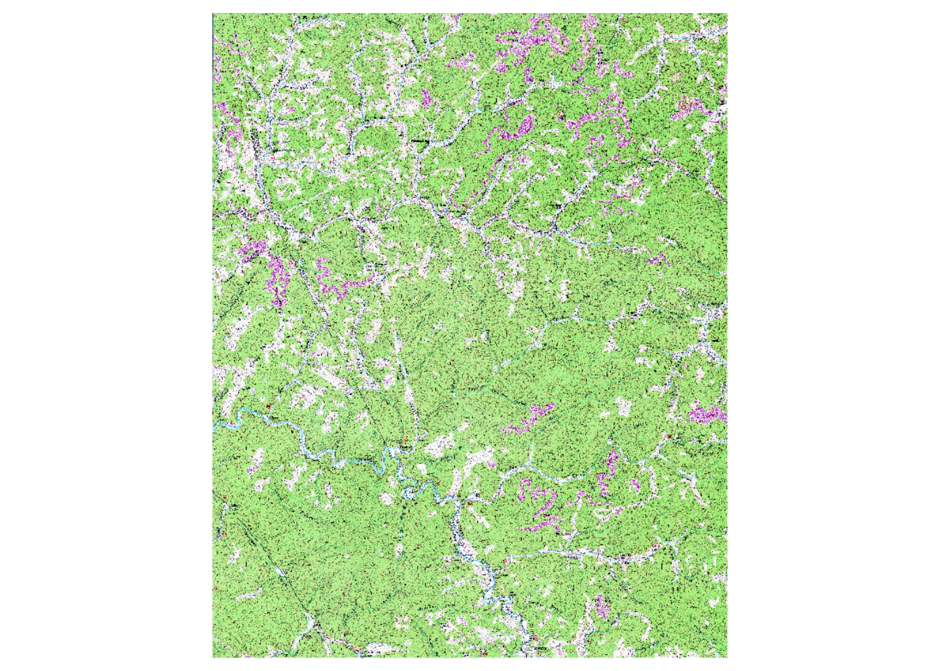
tm_shape(refT)+
    tm_raster(col.scale = tm_scale_categorical(labels = c("Not Mine",
                                                           "Mine"
                                                           ),
                                             values = c("gray80",
                                                         "salmon")),
            col.legend = tm_legend("Land Cover"))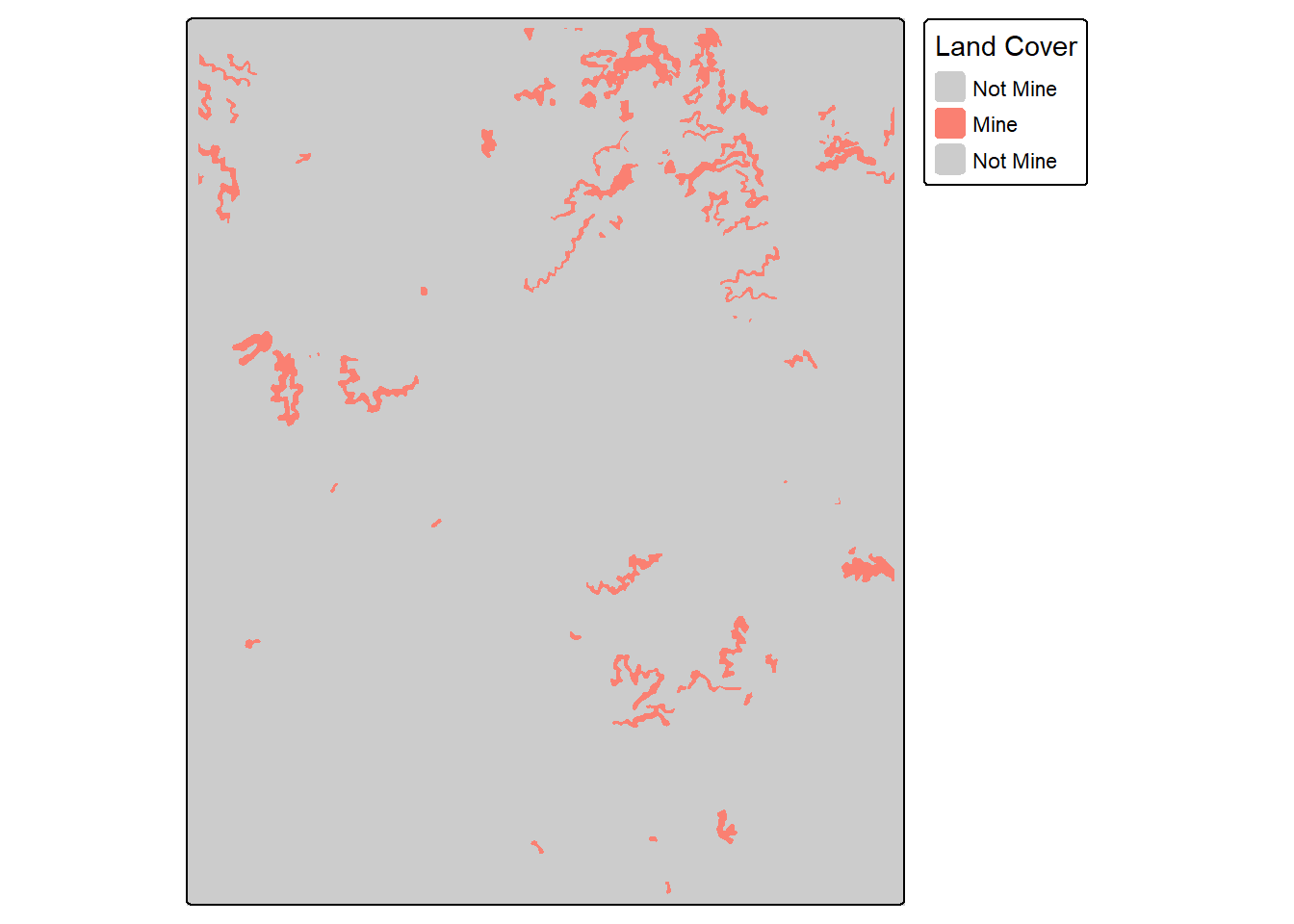
tm_shape(predT)+
    tm_raster(col.scale = tm_scale_categorical(labels = c("Not Mine",
                                                           "Mine"
                                                           ),
                                             values = c("gray80",
                                                         "salmon")),
            col.legend = tm_legend("Land Cover"))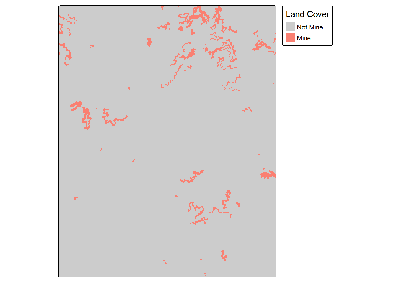
pntsIn2 <- terra::project(pntsTopo, terra::crs(refT))
refIsect <- terra::extract(refT, pntsIn2)
predIsect <- terra::extract(predT, pntsIn2)

resultsIn <- data.frame(ref=as.factor(refIsect$topoRef),
                        pred=as.factor(predIsect$topoPred))

resultsIn$ref <- forcats::fct_recode(resultsIn$ref,
                                   "Not Mine" = "0",
                                   "Mine" = "1")
resultsIn$pred <- forcats::fct_recode(resultsIn$pred,
                                   "Not Mine" = "0",
                                   "Mine" = "1")
myMetrics <- assessPnts(reference=bIn$ref,
predicted=bIn$pred,
multiclass=FALSE,
mappings=c("Not Mine", "Mine")
)
print(myMetrics)$Classes
[1] "Not Mine" "Mine"
$referenceCounts
Negative Positive
4822 178
$predictionCounts
Negative Positive
4840 160
$ConfusionMatrix
Reference
Predicted Negative Positive
Negative 4820 20
Positive 2 158
$Mets
OA Recall Precision Specificity NPV F1Score
Mine 0.9956 0.8876 0.9875 0.9996 0.9959 0.934915.6.4 Example 4: Use Raster Grids
The assessRaster() function allows for calculating assessment metrics from reference and prediction categorical raster grids as opposed to point locations or tables. Note that the grids being compared should have the same spatial extent, coordinate reference system, and number of rows and columns of cells.
predT <- terra::resample(predT, refT)myMetrics <- assessRaster(reference = refT,
predicted = predT,
multiclass = FALSE,
mappings = c("Not Mine", "Mine")
)
print(myMetrics)$Classes
[1] "Not Mine" "Mine"
$referenceCounts
Negative Positive
36022015 1301194
$predictionCounts
Negative Positive
36146932 1176277
$ConfusionMatrix
Reference
Predicted Negative Positive
Negative 35994704 152228
Positive 27311 1148966
$Mets
OA Recall Precision Specificity NPV F1Score
Mine 0.9952 0.883 0.9768 0.9992 0.9958 0.927515.7 Spatial Predictions
We will demonstrate using trained models to make predictions to full spatial extents in the next chapter. This is accomplished using geodl’s predictSpatial() function.
15.8 DTM Utilities
geodl provides some additional functionality for working with digital terrain models (DTMs). This section provides a brief introduction to this component of the package.
15.8.1 Land Surface Parameters (LSPs)
Many land surface parameters are calculated using local moving windows. Although packages such as terra and spatialEco already provide functionality for creating LSPs, as explored in Chapter 2, computation can be slow. Since torch implements moving windows in order to perform convolutional operations and because it supports GPU-based computation, opportunities arise to generate LSPs on the GPU using faster computation. geodl has made use of torch to implement several common LSPs as described in Table 15.2. Input data are converted to tensors, processing is performed on the GPU, and the resulting tensor is transferred back to the CPU and converted to a spatRaster() object, which can be saved to disk using writeRaster().
The examples below demonstrate creating the currently available LSPs, which include:
- topographic slope
- aspect or slope orientation measures (aspect, nortwardness, eastwardness, the transformed solar radiation aspect index (TRASP), and the site exposure index (SEI))
- hillshades and multi-directional hillshades
- topographic position index (TPI)
- surface curvatures (mean, profile, and planform)
The user is able to specify the size and/or shape of the moving window for several LSPs. For example, TPI can be calculated with a circular window with a user-defined radius or an annulus window with a user defined inner and outer radius. For the curvature measures, the input DTM can be smoothed using a circular moving window in order to remove the impact of local noise on the calculation.
Moving window radii are specified as cell counts as opposed to distances.
| Function | LSP | Description |
|---|---|---|
makeAspect() |
Topographic Aspect, Northwardness, Eastwardness, Site Exposure Index (SEI), or Topographic Radiation Aspect Index (TRASP) | Slope orientation in degrees or transformations |
makeSlope() |
Topographic Slope | Slope steepness in degrees |
makeHillshade() |
Hillshade or Multi-directional Hillshade | Visualization based on illumination using one or multiple sun positions |
makeTPI() |
Topographic Position Index (TPI) | Center Cell Elevation - Mean Elevation in Moving Window |
makeCrv() |
Mean, Profile, or Planform Curvature | Surface curvatures |
makeTerrainVisTorch() |
3-Band Terrain Visualization | Terrain visualization using hillslope TPI, slope, and local TPI (faster using torch) |
makeTerrainVisTerra() |
3-Band Terrain Visualization | Terrain visualization using hillslope TPI, slope, and local TPI (faster using terra) |
dtm <- terra::rast(str_glue(fldPth, "dtm.tif"))

slpR <- makeSlope(dtm,
                  cellSize=1,
                  writeRaster=TRUE,
                  outName=str_glue("{outPth}slp.tif"),
                  device="cuda")

aspR <- makeAspect(dtm,
                   cellSize=1,
                   flatThreshold=1,
                   mode= "aspect",
                   writeRaster=TRUE,
                   outName=str_glue("{outPth}asp.tif"),
                   device="cuda")

northR <- makeAspect(dtm,
                     cellSize=1,
                     flatThreshold=1,
                     mode= "northness",
                     writeRaster=TRUE,
                     outName=str_glue("{outPth}aspN.tif"),
                     device="cuda")

eastnessR <- makeAspect(dtm,
                        cellSize=1,
                        flatThreshold=1,
                        mode= "eastness",
                        writeRaster=TRUE,
                        outName=str_glue("{outPth}aspE.tif"),
                        device="cuda")

traspR <- makeAspect(dtm,
                     cellSize=1,
                     flatThreshold=1,
                     mode= "trasp",
                     writeRaster=TRUE,
                     outName=str_glue("outPth}trasp.tif"),
                     device="cuda")

seiR <- makeAspect(dtm,
                   cellSize=1,
                   flatThreshold=1,
                   mode= "sei",
                   writeRaster=TRUE,
                   outName=str_glue("{outPth}sei.tif"),
                   device="cuda")

hsR <- makeHillshade(dtm,
                     cellSize=1,
                     sunAzimuth=315,
                     sunAltitude=45,
                     doMD = FALSE,
                     writeRaster=TRUE,
                     outName=str_glue("{outPth}hs.tif"),
                     device="cuda")

hsMDR <- makeHillshade(dtm,
                       cellSize=1,
                       doMD = TRUE,
                       writeRaster=TRUE,
                       outName=str_glue("{outPth}hsMD.tif"),
                       device="cuda")

tpiC7 <- makeTPI(dtm,
                 cellSize=1,
                 innerRadius=2,
                 outerRadius=7,
                 mode="circle",
                 writeRaster=TRUE,
                 outName=str_glue("{outPth}tpiC7.tif"),
                 device="cuda")

tpiA3_11 <- makeTPI(dtm,
                    cellSize=1,
                    innerRadius=3,
                    outerRadius=11,
                    mode="circle",
                    writeRaster=TRUE,
                    outName=str_glue("{outPth}tpiA3_11.tif"),
                    device="cuda")

crvMn7 <- makeCrv(dtm,
                  cellSize=1,
                  mode="mean",
                  smoothRadius=7,
                  writeRaster=TRUE,
                  outName=str_glue("{outPth}crvMn7.tif"),
                  device="cuda")

crvPro7 <- makeCrv(dtm,
                   cellSize=1,
                   mode="profile",
                   smoothRadius=7,
                   writeRaster=TRUE,
                   outName=str_glue("{outPth}crvPro7.tif"),
                   device="cuda")

crvPln7 <- makeCrv(dtm,
                   cellSize=1,
                   mode="planform",
                   smoothRadius=7,
                   writeRaster=TRUE,
                   outName=str_glue("{outPth}crvPln7.tif"),
                   device="cuda")
dtm <- terra::rast(str_glue(fldPth, "dtm.tif"))
hsMDR <- terra::rast(str_glue(fldPth, "hsMD.tif"))
slpR <- terra::rast(str_glue(fldPth, "slp.tif"))
seiR <- terra::rast(str_glue(fldPth, "sei.tif"))
tm_shape(dtm)+
tm_raster(col.scale= tm_scale_continuous(values = "hcl.terrain2"),
col.legend = tm_legend("Elevation (meters)"))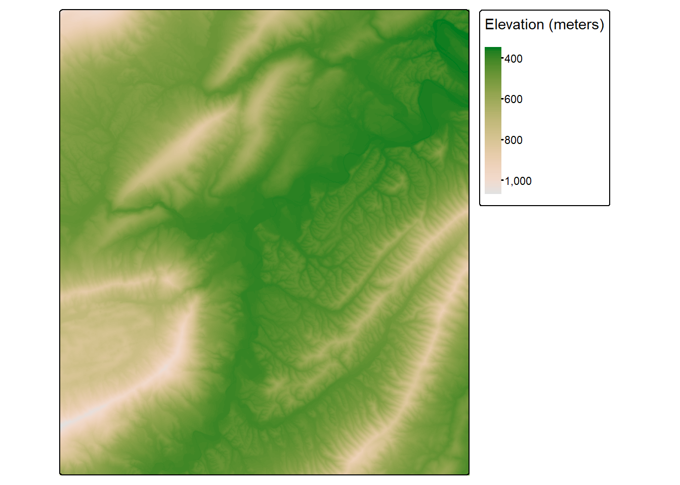
tm_shape(hsMDR)+
  tm_raster(col.scale= tm_scale_continuous(values = "-brewer.greys"),
            col.legend = tm_legend("Hillshade (Multi-Directional)"))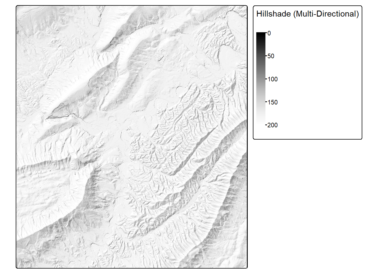
tm_shape(slpR)+
  tm_raster(col.scale= tm_scale_continuous(values = "brewer.yl_or_br"),
            col.legend = tm_legend("Slope (Degrees)"))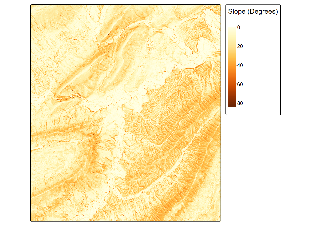
tm_shape(seiR)+
  tm_raster(col.scale= tm_scale_continuous(values = "-brewer.greys"),
            col.legend = tm_legend("Site Explosure Index (SEI)"))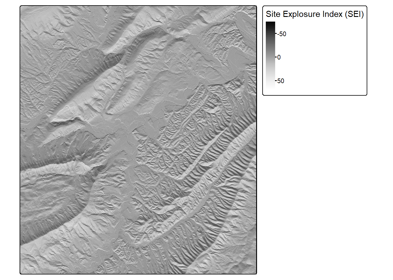
The makeTerrainDerivativesTerra() and makeTerrainDerivativesTorch() function creates a three-band raster stack from an input digital terrain model (DTM) of bare earth surface elevations. The first band is a topographic position index (TPI) calculated using a moving window with a circular radius. A larger radius is recommended to capture hillslope-scale topographic position. The second band is the square root of slope calculated in degrees. The third band is a TPI calculated using an annulus moving window. A smaller window is recommended to capture more local-scale topographic patterns. The TPI values are clamped to a range of -10 to 10 then linearly re-scaled from 0 and 1. The square root of slope is clamped to a range of 0 to 10 then linearly re-scaled from 0 to 1. Values are provided in floating point. This means of representing digital terrain data was proposed by Drs. Will Odom and Dan Doctor of the United States Geological Survey (USGS) and is discussed in the following publication, which is available in open-access:
Maxwell, A.E., W.E. Odom, C.M. Shobe, D.H. Doctor, M.S. Bester, and T. Ore, 2023. Exploring the influence of input feature space on CNN-based geomorphic feature extraction from digital terrain data, Earth and Space Science, 10: e2023EA002845. https://doi.org/10.1029/2023EA002845.
The code below provides an example of how to implement the makeTerrainDerivativesTorch() function. The dtm argument must be either a spatRaster object or a path and file name for a DTM on disk. Note that the vertical units should be the same as the horizontal units. The res parameter is used to specify the spatial resolution of the DTM data, which is required for calculations implemented internally. The DTM used in the example has a spatial resolution of 1-by-1 meters.
The output of this function is more meaningful for high spatial resolution digital terrain data (i.e., pixel sizes <= 5 m). The function returns the three-band raster as a spatRaster object and also writes the output to disk. We recommend saving the result as either a “.tif” or “.img” file.
The makeTerrainDerivativesTerra() produces the same result. However, computation does not make use of torch and GPU-based computation. As a result, it is generally slower than the torch-based implementation.
tVis <- makeTerrainVisTorch(dtm,
                            cellSize=1,
                            innerRadius=2,
                            outerRadius=5,
                            hsRadius=50,
                            writeRaster=TRUE,
                            outName=str_glue("{outPth}topoVisTorch.tif"),
                            device="cuda")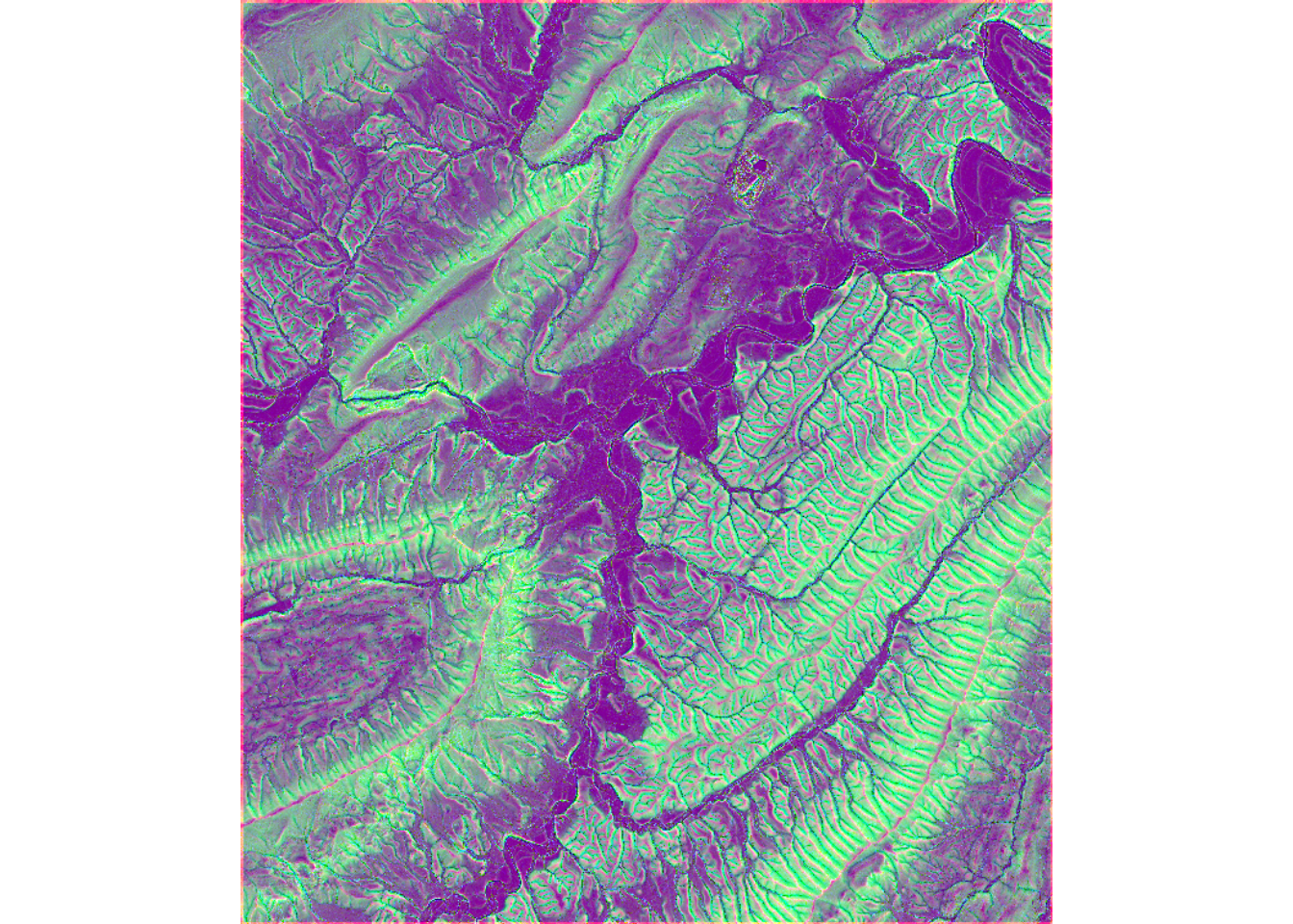
15.8.2 TerrainSeg Model
geodl also implements a means to perform semantic segmentation or feature extraction of geomorphic, landform, or archeological features using LSP predictor variables. The defineTerrainSeg() function prepends the module conceptualized in Figure 15.8 to a semantic segmentation model (either, UNet, MobileNetv2-UNet, UNet3+, or HRNet). This module calculates the following LSPs:
- Topographic slope
- Local topographic position index (TPI) using a small annulus moving window
- Multi-directional hillshade
- Planform curvature
- Profile Curvature
- Hillslope topographic position index (TPI) using a larger annulus moving window.
The user is able to define moving window sizes to parameterize the TPI calculations. Smoothing can be applied prior to calculating surface curvatures to reduce the impact of local noise. The hillshade is calculated with illumination from the north, south, east, and west. This is so that applying random rotations, as implemented with defineSegDataSet() or defineDynamicSegDataSet() will not impact the illumination. All values are clipped and re-scaled to a range of 0 to 1.
Once LSPs are calculated, rows and columns of cells are cropped to remove edge effects, and the stack of LSPs is then provided as predictor variables to the trainable semantic segmentation architecture.
It also supports generating LSPs at varying resolutions by implementing Gaussian spatial pyramid pooling at five different levels of smoothing. The user can choose whether or not to calculate Gaussian pyramids. If Gaussian pyramids are not used, 6 LSPs are passed to the trainable component of the model. If it is used, 31 LSPs are provided. Note that the hillslope-scale TPI is only calculated at the original resolution since it already uses a large window and is, as a result, already generalized.
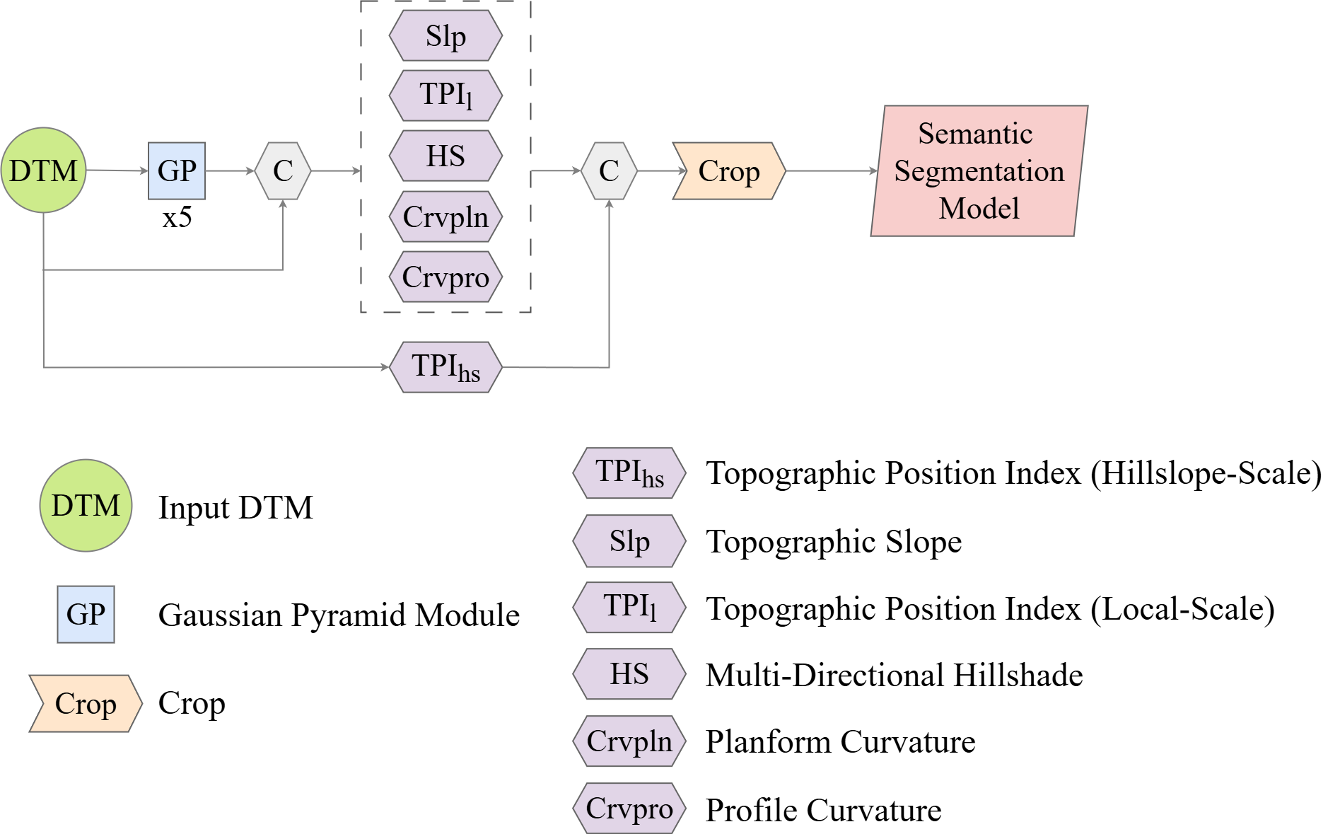
The code below shows how to instantiate, parameterize, and use the terrain segmentation model. In the example, we use the UNet3+ architecture and differentiate two classes. The local TPI uses an inner radius of 2 cells and an outer radius of 10 cells while the hillsope-scale TPI uses a 50 m circular radius. The DTM is smoothed using a 11 cell radius moving window prior to calculating the surface curvatures. We also use Gaussian pyramids, which results in passing 31 LSPs to the trainable component of the model.
The model expects input chips with spatial dimensions of 640-by-640. After the LSPs are calculated, 64 rows and columns are cropped from each side of the tensor. This results is LSPs with spatial dimensions of 512-by-512 being passed to the UNet3+ component.
terrainMod <- defineTerrainSeg(segModel="UNet3p",
                               nCls = 2,
                               cellSize = 1,
                               spatDim=640,
                               tCrop = 64,
                               doGP = TRUE,
                               innerRadius = 2,
                               outerRadius =10,
                               hsRadius = 50,
                               smoothRadius = 11,
                               actFunc="lrelu",
                               negative_slope = 0.01)$to(device="cuda")
t1 <- torch::torch_rand(c(12,1,640,640))$to(device="cuda")
p1 <- terrainMod(t1)p1$shape[1] 12 2 512 51215.9 Concluding Remarks
Now that we have explored the components of geodl, we are ready to implement the training, validation, and prediction workflow. This is the focus of the next chapter where we describe three separate workflows.
15.10 Questions
- Describe the structure and purpose of a squeeze and excitation module.
- Describe the structure and purpose of an attention gate module.
- Explain the purpose of the lambda, gamma, and delta terms in the unified focal loss framework.
- Describe the components and structure of an atrous spatial pyramid pooling (ASPP) module.
- How are the size of feature maps reduced in the spatial dimensions within the HRNet architecture?
- How are the size of the feature maps increased in the spatial dimensions within the HRNet architecture?
- Explain key differences and innovations of UNet3+ in comparison to base UNet.
- MobileNetv2 implements depthwise separable convolution. Explain how this is different from traditional convolution.
15.11 Exercises
Task 1
Using defineUNet(), instantiate an instance of a UNet-like architecture that meets the following criteria:
- Expects 7 input variables
- Differentiates 11 classes
- Uses the swish activation function throughout
- Uses attention gates along the skip connections
- Uses squeeze and excitation modules in the encoder with a reduction rate of 8.
- Produces the following number of feature maps for encoder blocks 1 through 4: 32, 64, 128, 128
- Produces 256 feature map in the bottleneck block
- Produces the following number of feature maps for decoder blocks 1 through 4: 128, 126, 64, 32
Task 2
Test the architecture on randomly generated data with a mini-batch size of 8 and spatial dimensions of 256x256.
Task 3
Use the countParams() function to count the number of trainable parameters in the model. How many total trainable parameters are included in the architecture? Which layer has the most trainable parameters?
Task 4
Using defineHRNet(), instantiate an instance of an HRNet-like architecture that meets the following criteria:
- Expects 8 input variables
- Differentiates 3 classes
- Generates 16 feature maps at level 1, 32 at level 2, 64 at level 3, and 128 at level 4
- Uses 128 feature maps in the decoder
- Generates 128 feature maps for each branch in the ASPP module
- Uses dilation rates of 3, 9, and 12 in the ASPP module
- Uses residual connections throughout
- Uses leaky ReLU activation functions with a negative slope term of 0.01
Task 5
Test the architecture on randomly generated data with a mini-batch size of 8 and spatial dimensions of 256x256.
Task 6
Use the countParams() function to count the number of trainable parameters in the model. How many total trainable parameters are included in the architecture?
Task 7
Instantiate an instance of the unified focal loss using defineUnifiedFocalLoss() configured as a focal Tversky loss with a gamma of 0.6 and a delta of 0.7 for a 7 class problem.
Task 8
Instantiate an instance of the unified focal loss using defineUnifiedFocalLoss() configured as a focal cross entropy loss with a gamma of 0.8 and a delta of 0.5, and class weights of c(0.1, 0.3, 0.4, 0.2) for a 4 class problem.