7 Random Forest
7.1 Topics Covered
- Prepare data as input to a random forest model
- Train random forest model
- Assess model predictions
- Compare different input feature spaces
- Use a random forest model to predict to raster data
- Assess variable importance using randomForest and permimp
- Assess variable importance using Boruta
- Assess variable importance using SHapley Additive exPlanations (SHAP) values
- Compare random forest and logistic regression models
- Create and interpret partial dependence plots
7.2 Introduction
Before discussing the more general tidymodels framework, we will investigate a specific package for implementing the random forest algorithm: the randomForest package. We will specifically implement a workflow to generate a probabilistic model of wetland occurrence based on topographic characteristics represented using land surface parameters (LSPs). This problem is framed as a binary classification task: “wetland” vs. “upland”. However, instead of making use of the “hard” predictions, we primarily make sure of the probabilistic estimates.
We implement the random forest algorithm with the randomForest package. The tidyverse is used for general data wrangling, terra is used for handling raster geospatial data, and recipes is used for data preprocessing. Accuracy assessment is implemented with yardstick and pROC. We explore several means to estimate variable importance using the permimp, Boruta, and fastshap/shapviz packages. Lastly, tmap is used to visualize our spatial data.
The random forest algorithm and its derivatives are implemented in R via several packages including randomForest, ranger, and party/partykit.
7.3 Data Preparation
We step through the process of creating a spatial prediction to map the likelihood or probability of palustrine forested/palustrine scrub/shrub (PFO/PSS) wetland occurrence using a variety of LSPs. The provided training.csv table contains 1,000 examples of PFO/PSS wetlands and 1,000 not PFO/PSS examples. The validation.csv file contains a separate, non-overlapping 2,000 examples equally split between PFO/PSS wetlands and not PFO/PSS wetlands. The columns in the provided tables are summarized in Table 7.1. We have also provided a raster stack (predictors.img) of all the predictor variables so that a spatial prediction can be produced. Since PFO/PSS wetlands should only occur in woody or forested extents, we have also provided a binary raster mask (for_mask.img) to subset the final result to only areas with woody for forested land cover. For this example, we use only a subset of the available predictor variables. Several of the variables were calculated using different moving window sizes. We only use the averaged versions here.
| Variable | Description |
|---|---|
| class | PFO/PSS ("wet") or not ("not") |
| cost | Distance from water bodies weighted by slope |
| crv_arc | Topographic curvature |
| crv_plane | Plan curvature |
| crv_pro | Profile curvature |
| ctmi | Compound topographic moisture index (CTMI) |
| diss_5 | Terrain dissection (11 x 11 window) |
| diss_10 | Terrain dissection (21 x 21 window) |
| diss_20 | Terrain dissection (41 x 41 window) |
| diss_25 | Terrain dissection (51 x 51 window) |
| diss_a | Terrain dissection average |
| rough_5 | Terrain roughness (11 x 11 window) |
| rough_10 | Terrain roughness (21 x 21 window) |
| rough_20 | Terrain roughness (41 x 41 window) |
| rough_25 | Terrain Roughness (51 x 51 window) |
| rough_a | Terrain roughness average |
| slp_d | Topographic slope in degrees |
| sp_5 | Slope position (11 x 11 window) |
| sp_10 | Slope position (21 x 21 window) |
| sp_20 | Slope position (41 x 41 window) |
| sp_25 | slope position (51 x 51 window) |
| sp_a | Slope position average |
The training and test sets are read in using read_csv() from readr, the dependent variable (“class”) and the subset of predictor variables are extracted using select() from dplyr, and all character columns are converted to factors. We use forcats to recode the class names. Lastly, we use recipes to re-scale all the predictor variables to a zero to one range using the recipe() –> prep() –> bake() sequence. Only the training set is used to define the transformations to avoid a data leak. Note that this normalization is not strictly necessary for random forest since it is not sensitive to different measurement scales.
The randomForest package requires traditional data frame objects as opposed to tibbles; as a result, we use data.frame() to convert the training and test tibbles to regular R data frames.
fldPth <- "gslrData/chpt7/data/"

predsToUse <- c("cost",
                "ctmi",
                "crv_plane",
                "crv_pro",
                "diss_a",
                "rough_a",
                "slp_d",
                "sp_a")

train <- read_csv(str_glue("{fldPth}training.csv")) |>
  select(class, predsToUse) |>
  mutate_if(is.character, as.factor)

test <- read_csv(str_glue("{fldPth}validation.csv")) |>
  select(class, predsToUse) |>
  mutate_if(is.character, as.factor)

train$class <- dplyr::recode(train$class,
                   "wet" = "Wetland",
                   "not" = "Upland")

test$class <- dplyr::recode(test$class,
                   "wet" = "Wetland",
                   "not" = "Upland")

myRecipe <- recipe(class ~ ., data = train) |>
  step_range(all_numeric_predictors(), min=0, max=1)

myRecipePrep <- prep(myRecipe, training=train)

trainP <- bake(myRecipePrep, new_data=NULL) |>
  data.frame()
testP <- bake(myRecipePrep, new_data=test) |>
  data.frame()
We next prepare the raster data. The stack of predictor variables are read in using rast() from the terra package, the bands are renamed to match the predictor variable names in the tabulated data, and the subset of predictor variables are extracted out using bracket notation. Since the tabulated data were re-scaled, it is also necessary to apply this same preprocessing step to the raster data for consistency. This is accomplished by extracting the raster values into a data frame, using bake() to process the data frame, then writing the resulting values back into the raster grid to replace the original values.
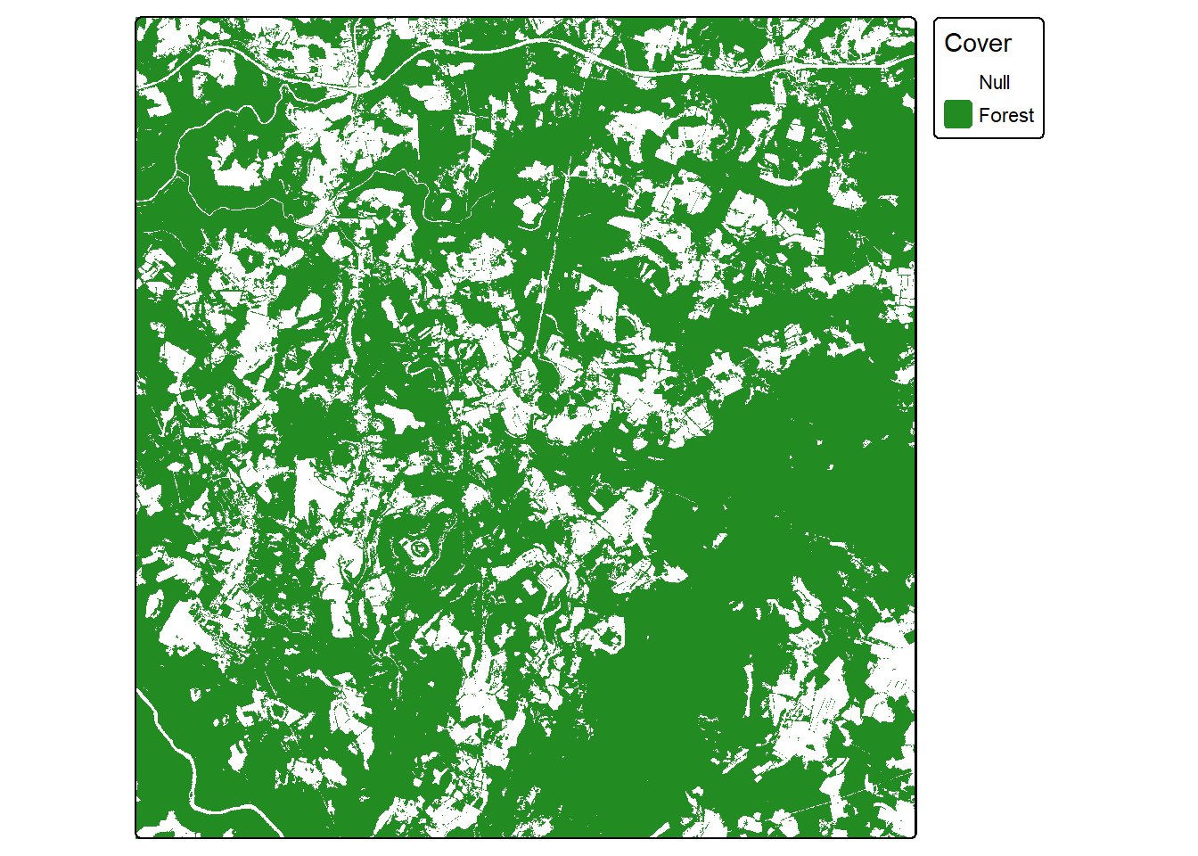
We also read in the forest mask. Areas outside of forested extents are coded to NA while forested areas are coded to 1.
Lastly, we visualize one predictor variable, topographic slope (“slp_d”) and the forest mask using tmap. This confirms that the slope variable has been rescaled to a 0 to 1 range.
predStk <- rast(str_glue("{fldPth}predictors.tif"))

names(predStk) <- c("cost",
                    "crv_arc",
                    "crv_plane",
                    "crv_pro",
                    "ctmi",
                    "diss_5",
                    "diss_10",
                    "diss_20",
                    "diss_25",
                    "diss_a",
                    "rough_5",
                    "rough_10",
                    "rough_20",
                    "rough_25",
                    "rough_a",
                    "slp_d",
                    "sp_5",
                    "sp_10",
                    "sp_20",
                    "sp_25",
                    "sp_a")

predStk <- predStk[[predsToUse]]

predStkDF <- as.data.frame(predStk, xy=FALSE, na.rm=FALSE)

predStkDFP <- bake(myRecipePrep, new_data=predStkDF)
predStk[] <- as.matrix(predStkDFP)

forMsk <- rast(str_glue("{fldPth}for_mask.tif"))tm_shape(predStk$slp_d)+
tm_raster(col.scale = tm_scale_continuous(values="tableau.brown"),
col.legend = tm_legend(title="Slope"))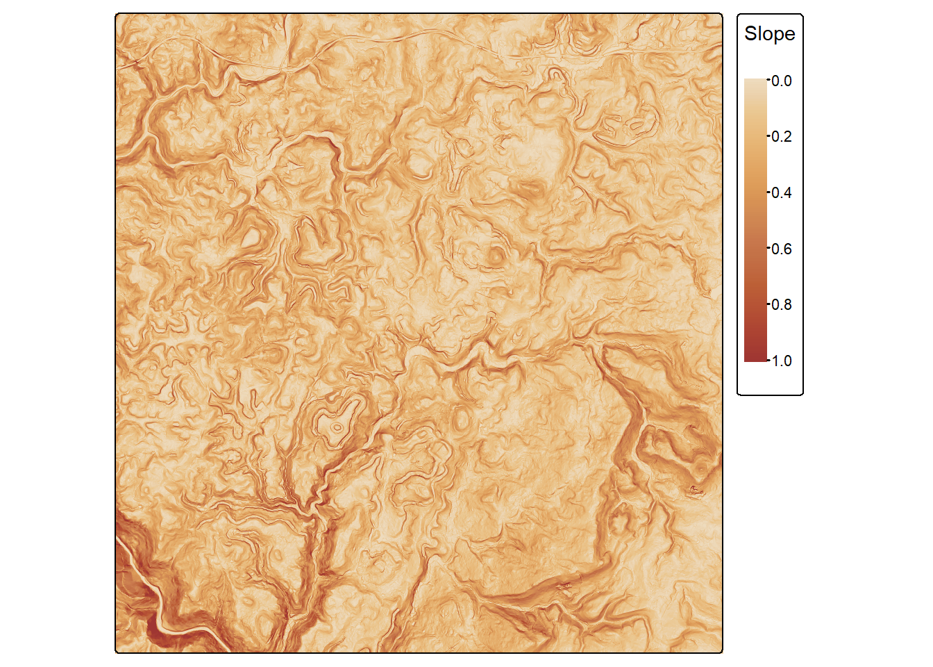
7.4 Base Model
7.4.1 Train Model
We first train a base model that uses all of the extracted predictor variables with the randomForest() function. The dependent variable is the last column in the table (“class”) while all other columns are predictor variables. We generate 501 trees in the ensemble, estimate variable importance, and calculate a confusion matrix and error rate using the out-of-bag (OOB) data for each tree. We also keep all the trees and in-bag estimates since these are necessary to implement some of the variable importance routines explored below.
Since there are only two classes, “Wetland” and “Upland”, we use an odd number of trees in the ensemble to avoid a tie. When more than two categories are differentiated, using an odd number of trees does not guarantee no ties, so we generally only recommend this for binary problems.
Calling the model prints some general information about it including the model call, number of trees in the model, and the number of random variables to select from at each decision node. Since we did not set this hyperparameter, the default was used. For a classification task, this is the square root of the number of total predictor variables rounded down. It is generally recommended to tune this hyperparameter; this is explored using tidymodels in a later chapter.
The OOB error rate is ~4.25%, which offers an estimate of model generalization since the OOB samples for each tree were not used to build that specific tree in the ensemble.
OOB error estimates are only unbiased if the training data are randomized and unbiased. There may also be some inflation if there is autocorrelation between the samples. Due to these issues, we recommend further assessing the model using a withheld set of samples from a different geographic extent.
set.seed(42)
mAll <- randomForest(y=trainP[,9],
                     x=trainP[,1:8],
                     ntree=501,
                     importance=T,
                     confusion=T,
                     err.rate=T,
                     keep.forest = TRUE,
                     keep.inbag = TRUE)

mAll
Call:
 randomForest(x = trainP[, 1:8], y = trainP[, 9], ntree = 501,      importance = T, keep.forest = TRUE, keep.inbag = TRUE, confusion = T,      err.rate = T)
               Type of random forest: classification
                     Number of trees: 501
No. of variables tried at each split: 2

        OOB estimate of  error rate: 4.25%
Confusion matrix:
        Upland Wetland class.error
Upland     949      51       0.051
Wetland     34     966       0.034
7.4.2 Explore Model
The randomForest package implementation of the random forest algorithm offers some additional output that can be used to interpret the model. For example, variable importance can be estimated using a permutation-based method. This involves shuffling the values for the predictor variable of interest while maintaining the alignment between the dependent variable and all the other predicts. For more important predictor variables, model performance should decrease more when random permutation is applied. This measure is referred to as the out of bag mean decrease in accuracy measure. Importance can also be assessed based on the mean decrease in the Gini index, which is the measure used to select optimal splitting rules. This method is not discussed here.
It has been documented that permutation-based estimates of variable importance, such as OOB mean decrease in accuracy, can be biased if predictor variables are correlated, when a mix of continuous and categorical predictor variables are used, and/or when the number of levels vary between different categorical predictor variables. As a result, we investigate other methods for assessing variable importance later in this chapter.
The varImpPlot() function is used to visualize variable importance estimates. Ignoring the issues mentioned above, distance from water bodies weighted by topographic slope (“cost”) is suggested to be the most important variable. Other important variables include topographic roughness (“rough_a”) and topographic dissection (“diss_a”).
Partial dependence plots characterize how the response varies with the values of a specific predictor variable. To calculate a partial dependence plot, the average value is used for all predictor variables other than the predictor variable of interest. For the predictor variable of interest, the original values are used. Relative to the class of interest, larger scores, as shown on the y-axis in the partial dependence plots below, indicate a higher likelihood of being predicted to the class of interest while the x-axis maps the original predictor variable values. To construct the plot using the partialPlot() function from randomForest, the user must provide the trained model, a dataset that contains the dependent and predictor variables, the name of the variable of interest, and the class of interest.
The two partial dependence plots generated are for distance from water bodies weighted by slope (“cost”) and topographic slope (“slp_d”) variables. The plots generally suggest that wetlands are more likely to occur in flatter areas near streams, which makes sense. The pattern for topographic slope is noisier, but the plot generally suggests that wetlands are more likely to occur in flatter areas.
As with variable importance, partial dependence plots can be misleading or biased if variables are highly correlated. Regardless, we do find them informative, especially when considering more general trends as opposed to local noise.
varImpPlot(mAll)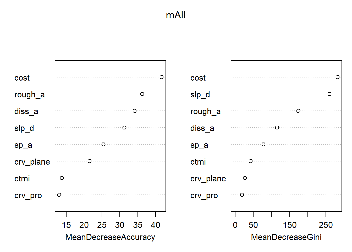
partialPlot(x=mAll,
            pred.data=trainP,
            x.var=cost,
            which.class="Wetland")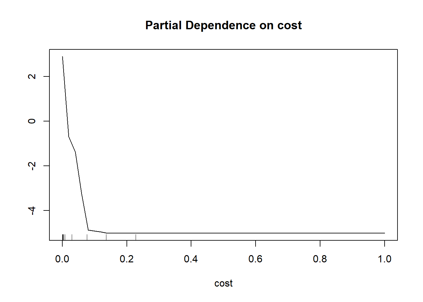
partialPlot(x=mAll,
            pred.data=trainP,
            x.var=slp_d,
            which.class="Wetland")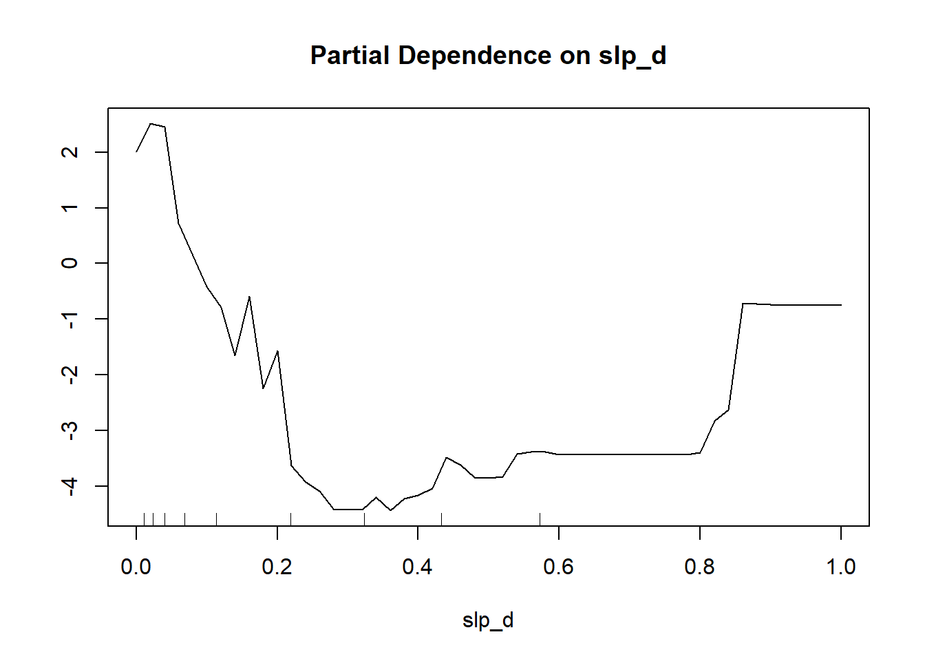
7.5 Compare Feature Spaces
We will now compare models using different features:
- All predictor variables
- Just topographic slope
- Just distance from water bodies weighted by slope
We do not need to train the model that used all predictor variables again since it was already created above. The two new models are trained in the following code block using R’s formula syntax to specify the model.
set.seed(42)
mSlp <- randomForest(class ~ slp_d,
                     data=trainP,
                   ntree=501,
                   importance=T,
                   confusion=T,
                   err.rate=T)

set.seed(42)
mCost <- randomForest(class ~ cost,
                      data=trainP,
                    ntree=501,
                    importance=T,
                    confusion=T,
                    err.rate=T)
We now compare the models based on their predictions to the withheld test data. This requires first obtaining predictions for all test samples using the different models. This can be accomplished using the predict() function. To compare the models based on the area under the receiver operating characteristic curve (AUCROC), we need to obtain the probabilistic or “soft” predictions as opposed to the predicted class labels or “hard” predictions. This requires setting the type argument to “prob”. To calculate overall accuracy, we need to obtain the “hard” predictions, which is accomplished using type="class".
mAllP <- predict(mAll,
                 testP,
                 index=2,
                 type="prob",
                 norm.votes=TRUE,
                 predict.all=FALSE,
                 proximity=FALSE,
                 nodes=FALSE) |>
  data.frame()

mSlpP <- predict(mSlp,
               testP,
               index=2,
               type="prob",
               norm.votes=TRUE,
               predict.all=FALSE,
               proximity=FALSE,
               nodes=FALSE) |>
  data.frame()

mCostP <- predict(mCost,
                testP,
                index=2,
                type="prob",
                norm.votes=TRUE,
                predict.all=FALSE,
                proximity=FALSE,
                nodes=FALSE) |>
  data.frame()
mAllC <- predict(mAll,
testP,
index=2,
type="class",
norm.votes=TRUE,
predict.all=FALSE,
proximity=FALSE,
nodes=FALSE) |>
data.frame()
mSlpC <- predict(mSlp,
testP,
index=2,
type="class",
norm.votes=TRUE,
predict.all=FALSE,
proximity=FALSE,
nodes=FALSE) |>
data.frame()
mCostC <- predict(mCost,
testP,
index=2,
type="class",
norm.votes=TRUE,
predict.all=FALSE,
proximity=FALSE,
nodes=FALSE) |>
data.frame()Next, we use the pROC package to calculate AUCROC for each model and the yardstick package to calculate overall accuracy. We write the results into a data frame along with the name of the model. We specifically used the predicted probabilities for the “Wetland” class since this is considered the positive case. The results generally suggest that the model that used all the predictor variables provided the best performance followed by the model that used only the distance from water bodies weighted by slope variable. The model using only topographic slope provided the poorest performance.
We also use the ggroc() function from pROC to plot the ROC curves for all 3 models in the same graph space. This function allows for generating ROC curve plots using ggplot2. We also make use of geom_abline() to add a the one-to-one line that represents random model performance. scale_color_manual() is used to assign unique colors to each ROC curve. The curves further highlight the strong performance of the model that used all predictor variables.
aucResults <- data.frame(case = c("All",
                                  "Slope",
                                  "Stream Cost Distance"),
                         auc = c(auc(roc(test$class, mAllP$Wetland)),
                                 auc(roc(test$class, mSlpP$Wetland)),
                                 auc(roc(test$class, mCostP$Wetland))),
                         oa = c(accuracy_vec(test$class, mAllC[,1]),
                                 accuracy_vec(test$class, mSlpC[,1]),
                                 accuracy_vec(test$class, mCostC[,1]))
)

aucResults |> ggplot(aes(x=auc, y=case))+
  geom_point(size=3, color="red")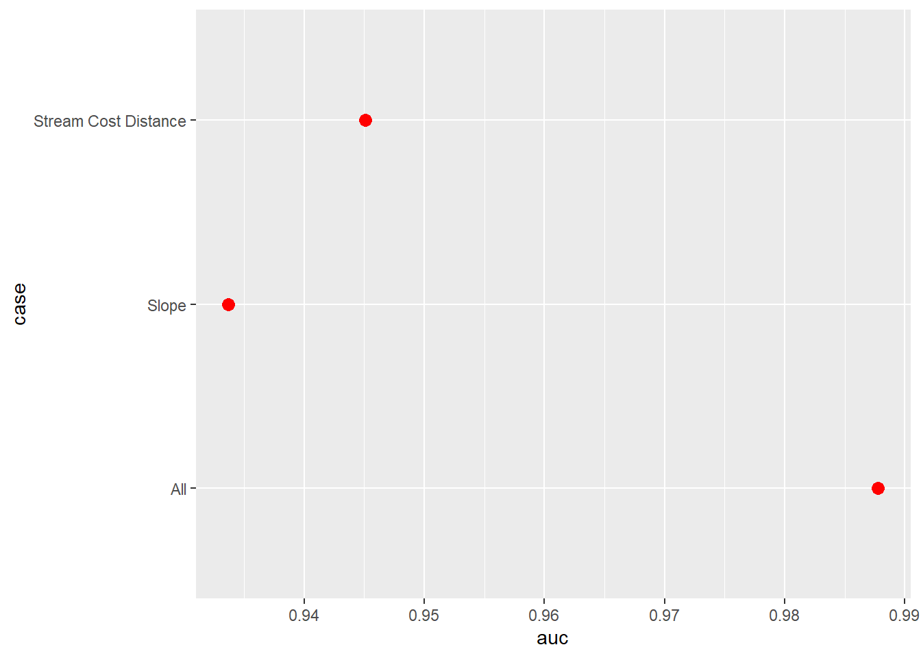
aucResults |> ggplot(aes(x=oa, y=case))+
  geom_point(size=3, color="red")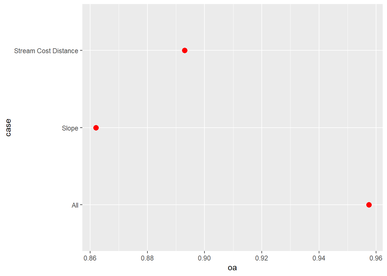
mAllROC <- roc(test$class, mAllP$Wetland)
mSlpROC <- roc(test$class, mSlpP$Wetland)
mCostROC<- roc(test$class, mCostP$Wetland)

ggroc(list(All=mAllROC,
           Slope=mSlpROC,
           Cost=mCostROC),
      lwd=1.2)+
  geom_abline(intercept = 1,
              slope = 1,
              color = "red",
              linetype = "dashed",
              lwd=1.2)+
  scale_color_manual(labels = c("All",
                                "Slope",
                                "Stream Cost Distance"),
                     values= c("#efd09e",
                               "#d2d8b3",
                               "#90a9b7"))+
  ggtitle("Model Comparison")+
  labs(x="Specificity", y="Sensitivity")+
  theme(axis.text.y = element_text(size=12))+
  theme(axis.text.x = element_text(size=12))+
  theme(plot.title = element_text(face="bold", size=18))+
  theme(axis.title = element_text(size=14))+
  theme(strip.text = element_text(size = 14))+
  theme(legend.title=element_blank())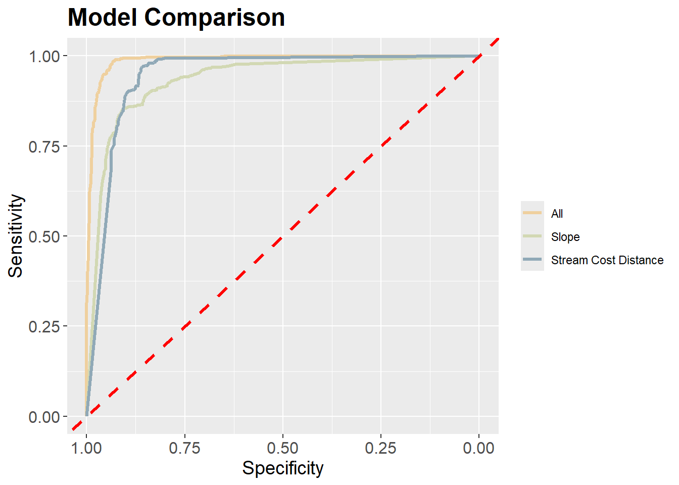
7.6 Predict to Raster Data
Once a model is trained, it can be used to generate map or model output by using it to make predictions to all raster grid cells within a spatial extent. Since the raster data have already been prepared above, we simply need to use the predict() function to make predictions to all raster cells in the grid. We obtain the probabilistic output for the wetland class. This is index 2 since “Wetland” is the second factor level. The resulting prediction is multiplied by the forest mask to recode all cells outside of forested extents to NA or to only maintain predictions within forested extents.
It is important that you know the correct order of the predictor variables in the raster stack since you must make sure that the correct variable is aligned to the correct layer in the stack. This is purely based on the band name matched to the predictor variable name. It is not required for the predictor variables to be in the same order in the raster stack as they are in the table used to train the model.
The final result is displayed using tmap with the masked out areas shown in gray and the predicted woodland or forested areas shown using a purple color ramp. Areas with a high predicted likelihood of wetland occurrence tend to occur closer to streams or waterbodies and in flatter areas, as expected. If you need to save the resulting prediction to disk, this can be accomplished using terra and the writeRaster() function.
rPred <- predict(predStk,
                 mAll,
                 type="prob",
                 index=2,
                 na.rm=TRUE,
progress="window")*forMsktm_shape(rPred)+
tm_raster(
col.scale = tm_scale_continuous(values="-parks.arches2",
value.na="lightgray"),
col.legend = tm_legend(title="PFO/PSS Wetland Probability"))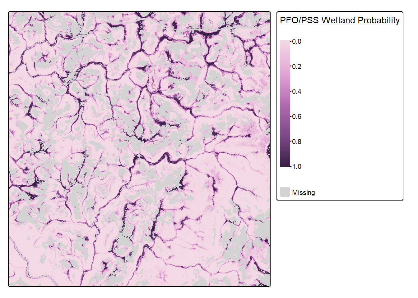
7.7 Variable Importance Estimation
As noted above, the default random forest predictor variable importance estimation method based on random permutation and the OOB mean decrease in accuracy measure can be misleading if the predictor variables are correlated. The permimp package offers an enhanced means to estimate variable importance for a random forest model that takes into account variable correlation.
The permimp() function performs this calculation. If conditional=TRUE a conditional importance is estimated. This is generally interpreted as a measure of the importance of the variable given the the other variables in the model. In other words, it estimates the additional information provided by the variable given the other variables in the feature space. In contrast, if conditional=FALSE is used, a more marginal estimate of importance is generated. This is meant to measure the importance of the variable regardless of the other variables used in the model. In other words, it measures how well the predictor variable predicts or estimates the dependent variable. If there is no correlation between the predictor variables, conditional and marginal importance are equivalent. Further, conditional and marginal importance are often conceptualized as end members of a continuum.
There is not a correct measure of variable importance. The optimal measure depends on what you are attempting to quantify. If you are more interested in the added value of including the variable given the other variables in the feature space, conditional importance may be of more interest. If you are more interested in how well the variable predicts the dependent variable regardless of the other variables in the model, marginal importance may be of more interest.
Once variable importance has been estimated, it can be plotted using plot().
Note that the perimp() function can be applied to models fit using the randomForest, ranger, and party/partykit packages. The party/partykit packages provide the cforest() function, which fits conditional inference trees, a modification of random forest that considers variable correlation. We generally prefer to use this method when we are specifically interested in quantifying variable importance. However, here we use our normal random forest model since it was already trained above and to align with the rest of the material in the chapter.
Conditional importance takes longer to calculate than marginal importance since the implementation is more computationally intensive.
The results of this analysis are visualized as box plots using the subsequent code blocks. Both methods still suggest that the distance from water bodies weighted by slope is an important variable. The marginal importance estimates are generally more varied than the conditional estimates.
plot(impReC,
     type = "box",
     horizontal = TRUE)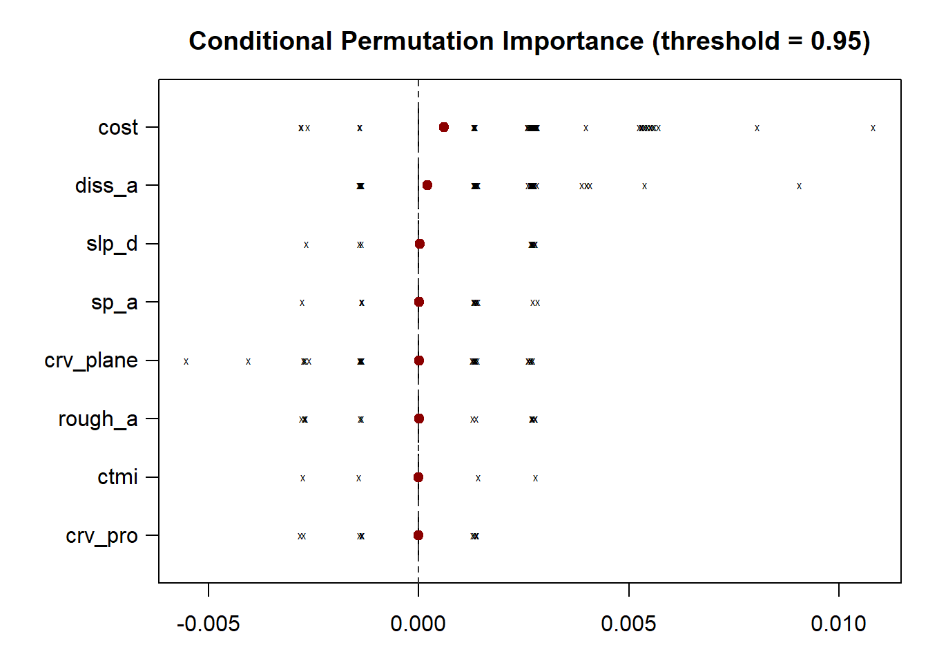
plot(impReUC,
     type = "box",
     horizontal = TRUE)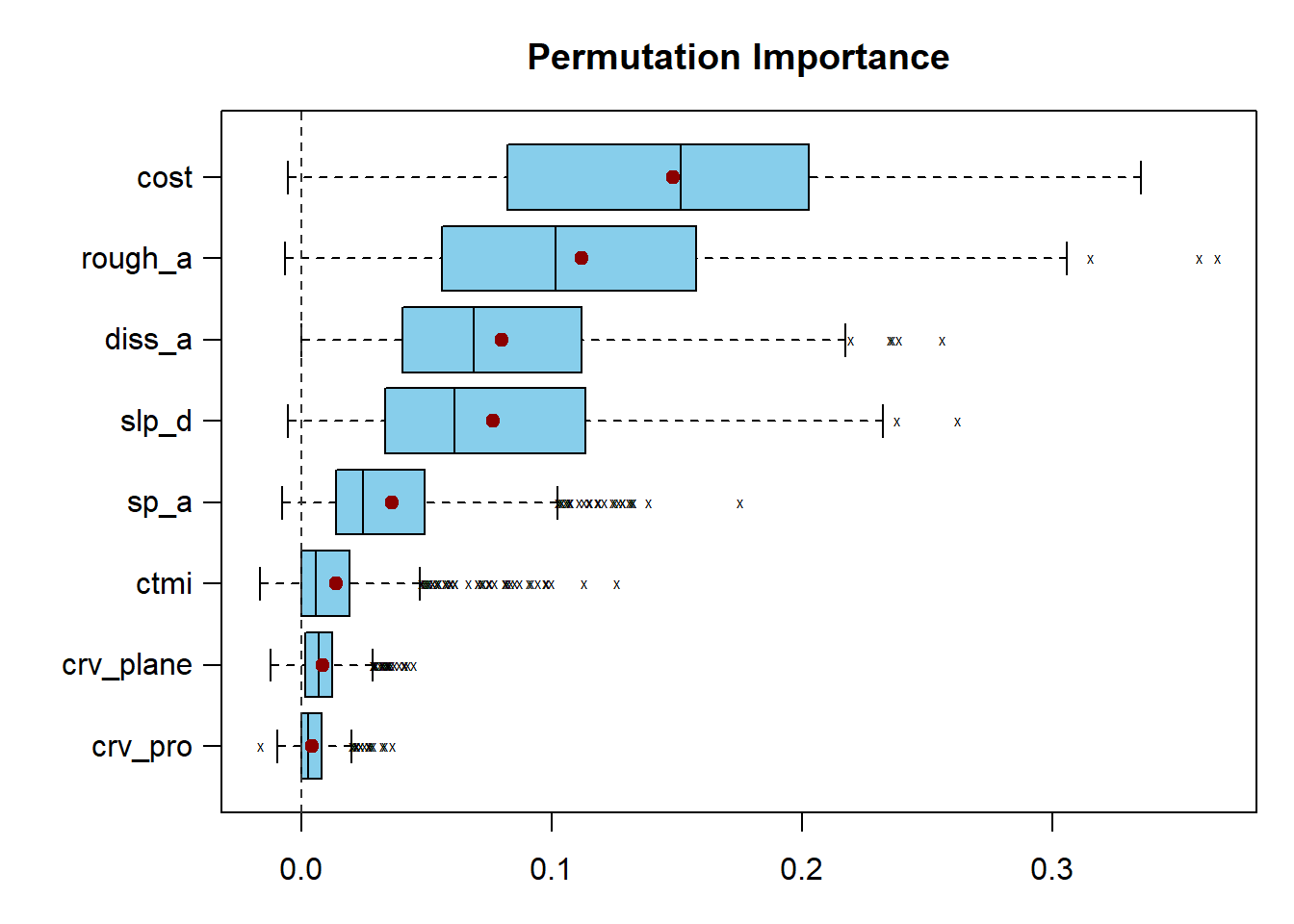
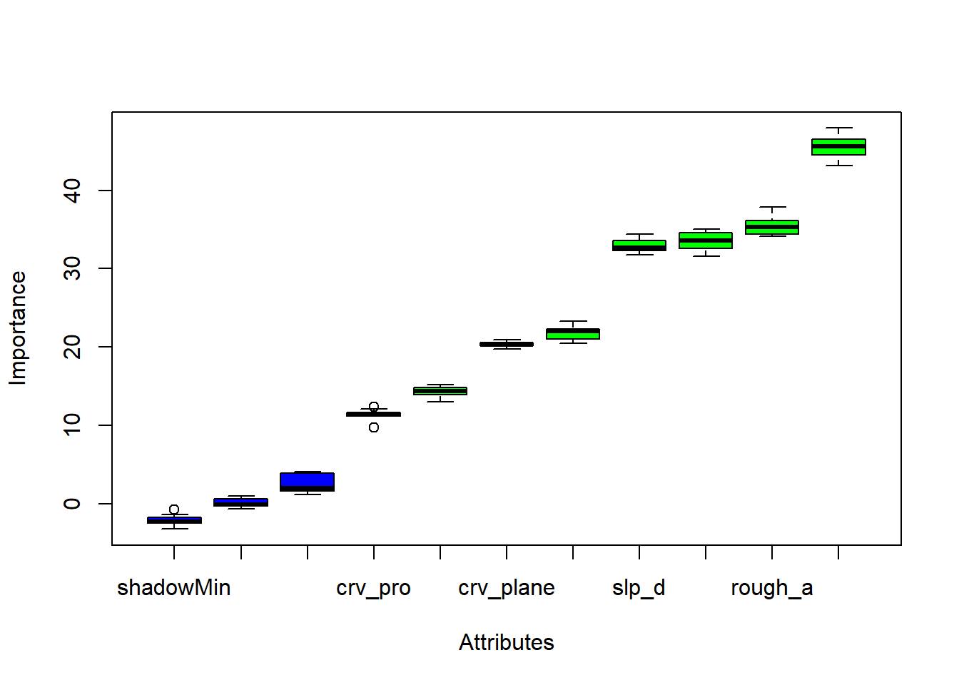
Another means to estimate variable importance is the Boruta method. This requires comparing the variables to permuted shadow variables to categorize each predictor variables as “not important,” “tentatively important,” or “important.” This method is implemented with the Boruta package, and is demonstrated in the following code block.
7.8 Compare to Logistic Regression
Other than comparing different feature spaces, an analyst may also want to compare different algorithms or modeling methods. In this section, we compare our random forest model to a logistic regression model. Specifically, we are interested in quantifying whether the more complex random forest model outperforms a simpler and more interpretable model.
Since logistic regression is a type of generalized linear model (GLM), it can be fit using the base R glm() function and using the logit link function. When using this implementation, the positive case can be assigned a value of 1 and the background case can be assigned a value of 0. Alternatively, if factor levels are used, the second factor level is assumed to be the positive case. Since this is the configuration for our current problem, we do not need to augment the representation of the dependent variable.
The following code block trains a logistic regression model, uses it to make predictions for the withheld test data, and calculates accuracy assessment metrics. Using the logistic regression model to make predictions returns the estimated probabilities relative to the positive case as a vector equal in length to the number of test samples. In order obtain a “hard” classification, we must pick a decision threshold. In our example, we use 0.5; however, this may not be optimal. A different decision threshold could be selected based on false positive and false negative rates. However, 0.5 is adequate for our example.
Our results generally suggest that the random forest model outperformed logistic regression. However, the differences were not dramatic. Comparing the results obtain here to those obtained above using different feature spaces, for this specific task the feature space generally had a larger impact on model performance than the algorithm used. This is further highlighted by comparing the ROC curves.
mLR <- glm(
  class ~ .,     # formula: response ~ predictors
  data   = trainP,
  family = binomial(link = "logit")
)

mLRP <- predict(mLR,
                testP,
                type = "response")

mLRC <- factor(ifelse(mLRP > 0.5, "Wetland", "Upland"))

aucResults <- data.frame(case = c("Random Forest",
                                  "Logistic Regression"),
                         auc = c(auc(roc(test$class, mAllP$Wetland)),
                                 auc(roc(test$class, mLRP))),
                         oa = c(accuracy_vec(test$class, mAllC[,1]),
                                 accuracy_vec(test$class, mLRC))
                         )

aucResults |> ggplot(aes(x=auc, y=case))+
  geom_point(size=3, color="red")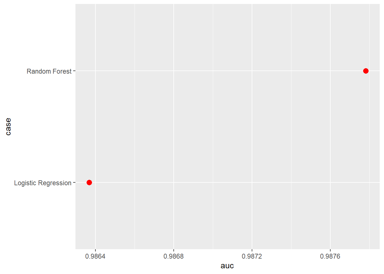
aucResults |> ggplot(aes(x=oa, y=case))+
  geom_point(size=3, color="red")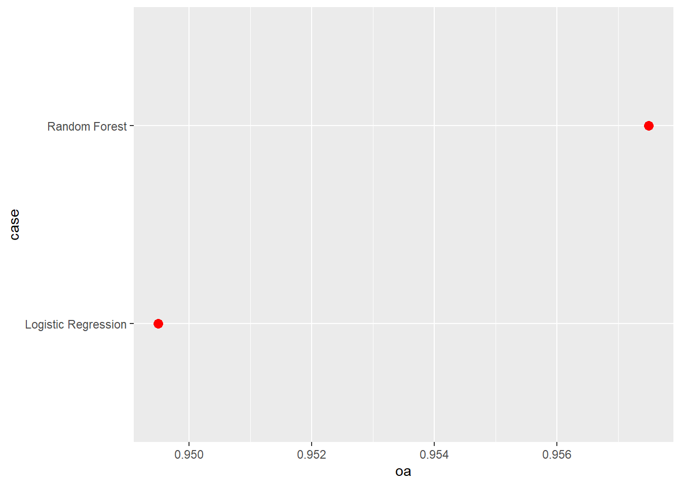
mRFROC <- roc(test$class, mAllP$Wetland)
mLRROC <- roc(test$class, mLRP)

ggroc(list(RF=mRFROC,
           LR=mLRROC),
      lwd=1.2)+
  geom_abline(intercept = 1,
              slope = 1,
              color = "red",
              linetype = "dashed",
              lwd=1.2)+
  scale_color_manual(labels = c("Random Forest",
                                "Logistic Regression"),
                     values= c("#efd09e",
                               "#90a9b7"))+
  ggtitle("Model Comparison")+
  labs(x="Specificity", y="Sensitivity")+
  theme(axis.text.y = element_text(size=12))+
  theme(axis.text.x = element_text(size=12))+
  theme(plot.title = element_text(face="bold", size=18))+
  theme(axis.title = element_text(size=14))+
  theme(strip.text = element_text(size = 14))+
  theme(legend.title=element_blank())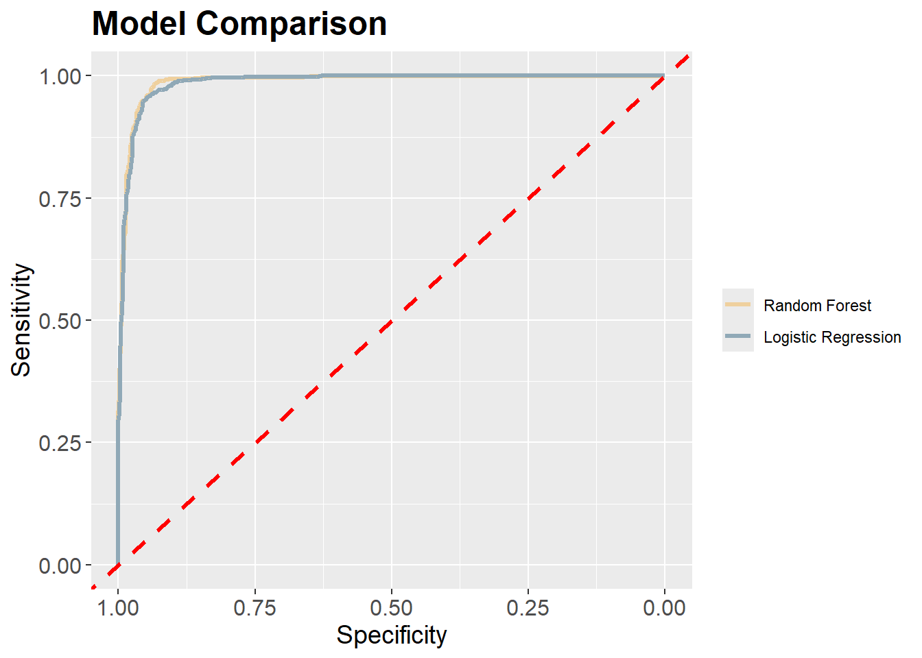
7.9 SHAP
You may be interested in using a model-agnostic means to assess variable contribution or importance, both globally and for individual predictions. One potential means to accomplish this is SHapely Additive exPlanations (SHAP). Grounded in cooperative game theory, this method attempts to quantify how the prediction changes when the predictor variable of interest is added to all possible combinations of the other predictor variables in the set. SHAP is implemented in R via the fastshap package while the shapvis package provides tools for visualizing the results.
The following code demonstrates the calculation of SHAP values. We first re-fit a random forest model using the ranger package as opposed to randomForest since we have found that this works better with the fastshap implementation.
We then obtain a local estimation for a single sample from the test set, specifically the data point at row 100, which is an example of a wetland as opposed to an upland. The generated plot is termed a waterfall plot, and the number associated with each variable represents the SHAP value associated with it. These values are added to the average prediction for the dataset, in this case 0.50, to obtain the prediction for the observation, which is 0.99 for this sample.
Another means to visualize the result is a force plot. In the example, the text above the arrows indicate the predictor variable values for the sample while the text inside the arrows indicate the SHAP values. Generally, these values can be conceptualized as the relative weight of evidence provided by each variable. If the arrow points to the right, the predictor variable supports the prediction to the wetland class. If it points to the left, it supports prediction to the background or upland class. For the example data point, all predictor variables support predicting the sample to the wetland case with the distance from streams weighted by slope, topographic roughness, and topographic slope having the largest impact on the prediction.
pfun <- function(object, newdata) {  # prediction wrapper
  unname(predict(object, data = newdata)$predictions[, "Wetland"])
}

exL <- fastshap::explain(rfMod,
                         X=testP[,1:8],
                         pred_wrapper=pfun,
                         newdata = testP[100,1:8],
                         nsim=10000,
                         adjust=TRUE)

baseline <- mean(pfun(rfMod,
                      newdata = trainP))

obS <- sum(exL)

shv <- shapviz(exL,
               X = trainP[400,1:9],
               baseline = baseline)
sv_waterfall(shv)+
  theme_bw(base_size=16)+
  scale_x_continuous(expand=c(0,0))+
  labs(x="SHAP value", y="")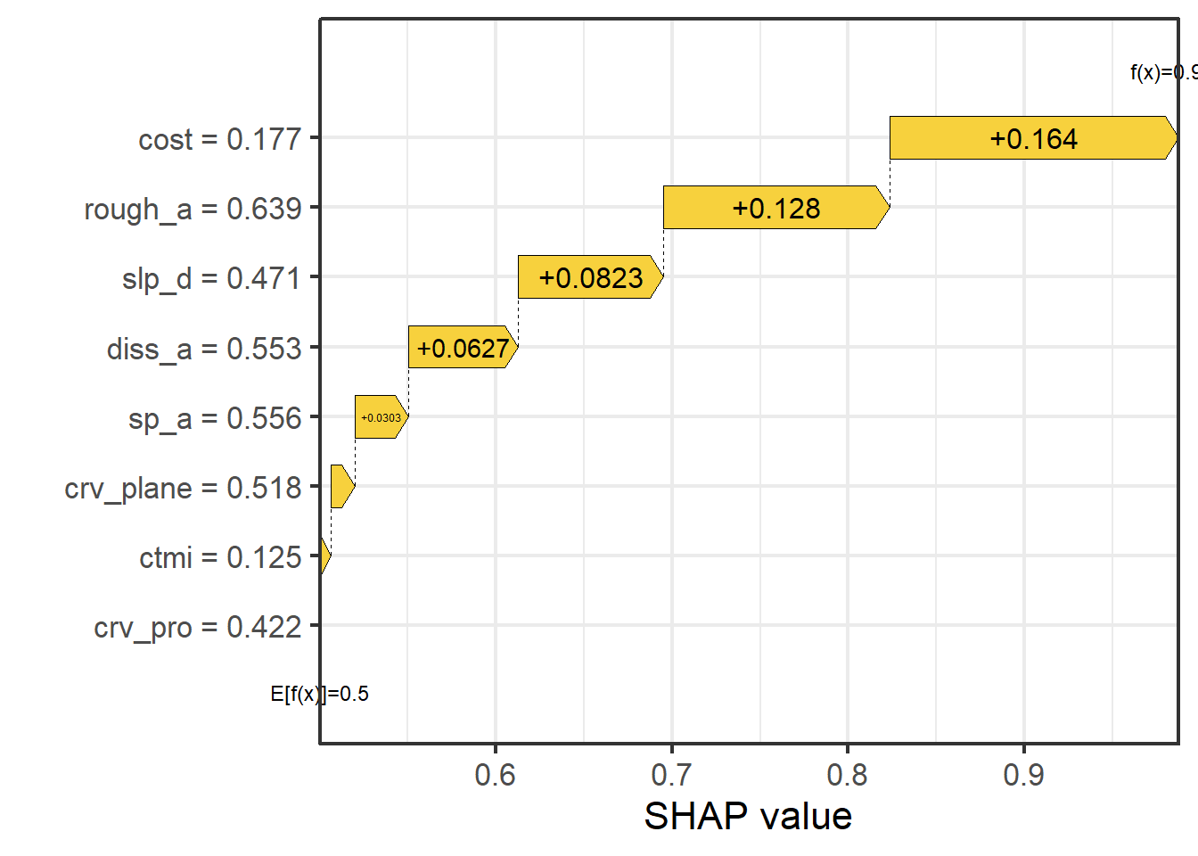
sv_force(shv)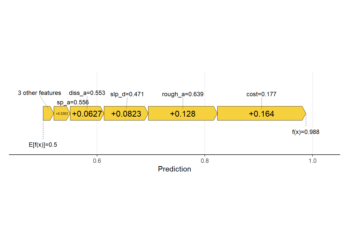
It is also possible to obtain global estimates of variable importance, which are estimated as the mean absolute value of SHAP values for a variable across all predictions. It is also possible to generate partial dependence plots based on SHAP values.
set.seed(42)  # for reproducibility
ex.t1 <- fastshap::explain(rfMod,
                           X = testP[,1:8],
                           pred_wrapper = pfun,
                           nsim = 100,
                           adjust = TRUE,
                           shap_only = FALSE)

shv.global <- shapviz(ex.t1)
sv_importance(shv)+
  theme_bw(base_size=16)+
  scale_x_continuous(expand=c(0,0))+
  scale_fill_manual(values = c("#444444","#bbbbbb"))+
  labs(x="Mean absolute SHAP value", y="")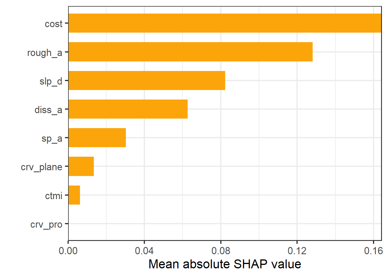
sv_dependence(shv.global, v = "cost", color_var=NULL, color="black")+
  theme_bw(base_size=16)+
  scale_x_continuous(expand=c(0,0))+
  labs(y="SHAP value", x="Topographic slope")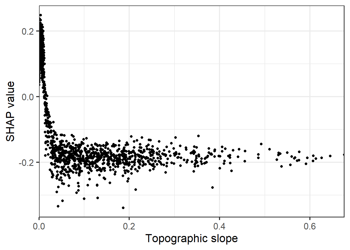
sv_dependence(shv.global, v = "slp_d", color_var=NULL, color="black")+
  theme_bw(base_size=16)+
  scale_x_continuous(expand=c(0,0))+
  labs(y="SHAP value", x="Heat load index (HLI)")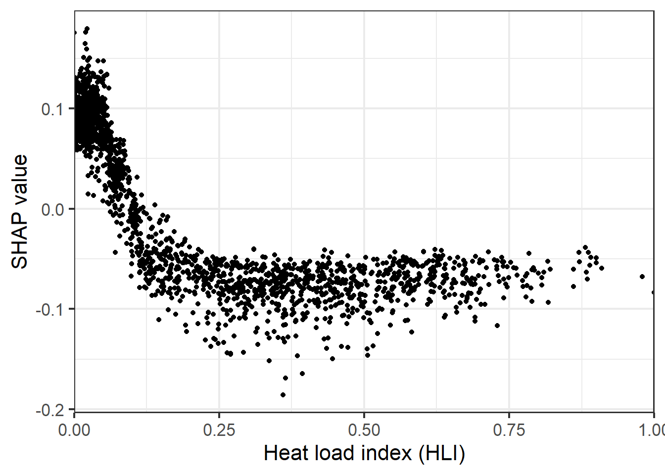
sv_waterfall(shv.global)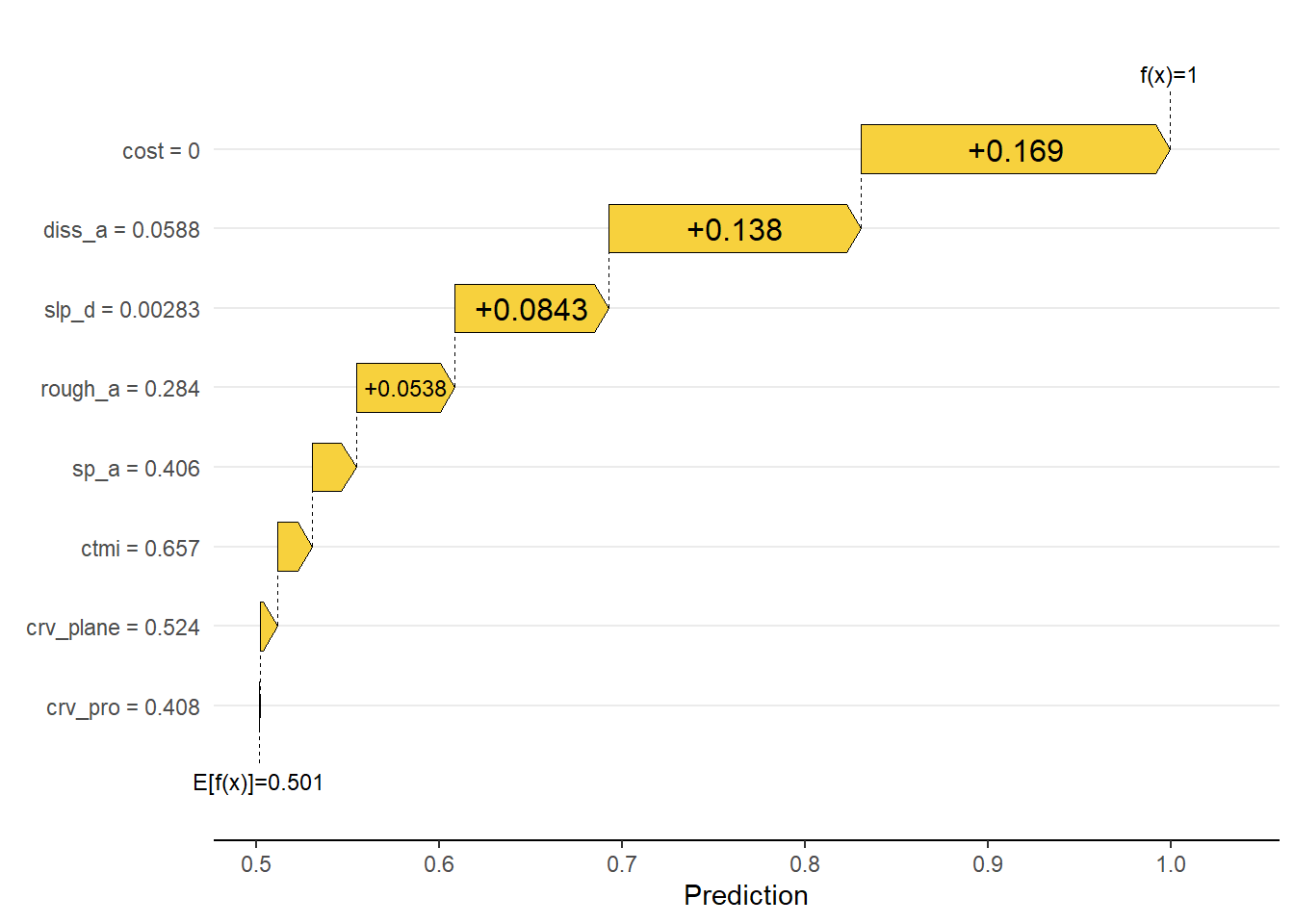
Some issues with SHAP values are that they can be computationally intensive to calculate (fastshap implements a faster approximation) and that they are impacted by predictor variable correlation.
7.10 Concluding Remarks
Now that we have discussed the full machine learning modeling process, we will investigate how it has been standardized in R using the tidymodels environment.
7.11 Questions
- Explain the difference between bagged decision trees, boosted decision trees, and random forest.
- For a classification task, how is the final classification obtained from the ensemble of single decision tree results?
- For a regression task, how is the final value obtained from the ensemble of single decision tree results?
- Explain the Gini impurity index and how is it used within random forests to determine an optimal splitting criterion.
- Is it necessary to re-scale all numeric predictor variables to be on the same scale when using random forest? Explain you answer.
- Explain how variable importance is assessed using the mean decrease in out-of-bag error metric as originally implemented in random forests.
- Explain the difference between conditional and marginal importance.
- Explain how a partial dependence plot for a single predictor variable is calculated.
7.12 Exercises
The goal of this exercise is to generate a model to predict the likelihood of landslide occurrence for raster cells within the Valley and Ridge physiographic province of West Virginia using topographic predictor variables. You have been provided with the following files in the exercise folder for the chapter.
- chpt7.gpkg/lsPnts: point locations representing landslide locations and pseudo-absence locations where predictor variables have been extracted
- stk.tif: raster stack of predictor variables
The following digital terrain model (DTM) derived land surface parameter (LSP) predictor variables have been provided. Other than elevation, the LSPs were calculated at three different window sizes.
- “elev”: elevation in meters
- “slp1”/“slp2”/“slp3”: topographic slope in degrees
- “sar1”/“sar2”/“sar3”: surface area ratio (SAR)
- “tri1”/“tri2”/“tri3”: topographic roughness index (TRI)
- “tpi1”/“tpi2”/“tpi3”: topographic position index (TPI)
- “diss1”/“diss2”/“diss3”: topographic dissection index
The “class” column differentiates landslides (“slpF”) from pseudo-absence samples (“not”).
Perform the following operations to train, validate, and use the model.
Preparation
- Read in the vector point layer, convert all character columns to factors, and drop the geometry information. Drop the “elev” column (you will not use this as a predictor variable).
- Read in the raster grid.
- Extract 1,000 examples each for the landslide and pseudo-absence classes using random sampling with replacement to serve as a training set. This can be accomplished using dplyr or rsample.
- Extract all remaining samples as a test set.
- Convert the training and test tables from tibbles to data frames (the randomForest package does not always work well with tibbles).
- Rename the raster bands to match the predictor variable columns in the table. They are in the same order.
Train Model
- Train the random forest model using the
randomForest()function from the randomForest package. The “class” column should be the dependent variable while all other columns should be predictor variables. Use the following settings:ntree = 501importance = TRUEconfusion = TRUEerr.rate = TRUEkeep.forest = TRUEkeep.inbag = TRUE
Explore Model
- Print the model summary. What was your out-of-bag error rate? Discuss omission and commission error rates.
- Use the
varImpPlot()function to generate a graph of estimated variable importance. - Use the
partialPlot()to generate partial dependence plots for the “slp1” and “diss1” variables. - Discuss your results. What variables were estimated to be most important in the model? What values of slope and dissection are most correlated with landslide occurrence?
Use Model
- Use your trained model to make predictions for each cell in the provided raster stack. Specifically, obtain the estimated probabilities for the landslide class.
- Plot the prediction using tmap.
Compare Models
- Train another model that uses only the “slp1” predictor variable. Use the same settings as the model with all predictor variables.
- Use both models to predict the test data to obtain both probabilistic and “hard” predictions.
- Using the predictions and provided labels, calculate overall accuracy, area under the precision-recall (AUCPR) curve, and area under the receiver operating characteristic curve (AUCROC).
- Plot the ROC curves for each model in the same plot space using
ggroc(). - Use the results to compare the models. Did the model using all predictor variables outperform the slope-only model?