16 Geospatial Semantic Segmentation Workflows
16.1 Topics Covered
- Prepare data for use in a geodl workflow
- Instantiate datasets and dataloaders
- Use luz to implement a training loop
- Train using pre-generated chips and associated masks
- Train using dynamically generated chips and associated masks
- Assess generated models and visualize results
- Use trained models to generate spatial predictions for new data
16.2 Introduction
geodl is still actively being developed. We recommend installing it from GitHub as opposed to CRAN. This can be accomplished using devtools as follows:
devtools::install_github("maxwell-geospatial/geodl")
In the last chapter, we described the functionality of the geodl package. In this chapter, we use its components to implement complete deep learning (DL) workflows. In the first workflow, we use the vfillDLMini dataset, which includes a set of pre-built image chips and associated masks. The goal is to extract valley fill face anthropocentric geomorphic features using digital terrain model (DTM)-derived land surface parameter (LSP) predictor variables. Valley fill faces are remnants of surface coal mine reclamation resulting from placing displaced overburden rock material in mine-adjacent valleys. Three predictor variables are included. The first band is a topographic position index (TPI) calculated using a moving window with a 50 m circular radius.The second band is the square root of slope calculated in degrees. The third band is a TPI calculated using an annulus moving window with an inner radius of 2 meters and an outer radius of 5 meters. The TPI values are clamped to a range of -10 to 10 then linearly rescaled from 0 and 1. The square root of slope is clamped to a range of 0 to 10 then linearly rescaled from 0 to 1. Values are provided in floating point. This means of representing digital terrain data was proposed by Drs. Will Odom and Dan Doctor of the United States Geological Survey (USGS) and is discussed in the following publication, which is available in open-access:
Maxwell, A.E., W.E. Odom, C.M. Shobe, D.H. Doctor, M.S. Bester, and T. Ore, 2023. Exploring the influence of input feature space on CNN-based geomorphic feature extraction from digital terrain data, Earth and Space Science, 10: e2023EA002845. https://doi.org/10.1029/2023EA002845.
These data can be downloaded at this link. The dataset is ~5 GB compressed.
The second workflow explores the same task. However, we now use the raw input DTM data, generate chips dynamically, and use the TerrainSeg framework that incorporates both the generation of LSPs and semantic segmentation into the model architecture. These data are available at this link. Note that this is a large datasets (~12 GB compressed).
The first two workflows explore a binary classification problem. The final workflow explores a multiclass classification problem focused on land cover mapping. We specifically use version 1 of the landcover.ai dataset, which is available at this link. Five classes are differentiated: Background, Building, Woodland, Water, and Road. The data originators provide a Python script to split the images and associated raster masks into 512x512 cell chips and have already defined training, validation, and testing partitions, which are listed into provided CSV files. The processing script is also available at the link provided above. The data were introduced in the following paper:
Boguszewski, A., Batorski, D., Ziemba-Jankowska, N., Dziedzic, T. and Zambrzycka, A., 2021. LandCover. ai: Dataset for automatic mapping of buildings, woodlands, water and roads from aerial imagery. In Proceedings of the IEEE/CVF conference on computer vision and pattern recognition (pp. 1102-1110).
16.3 Workflow 1: Valley Fill Faces (With Chips)
16.3.1 Preparation
We begin by reading in the required libraries. Other than geodl, we read in the tidyverse, terra, sf, torch, luz, tmap, and tmaptools. We also set the path to our downloaded version of the vfillDLMini dataset.
Remember to extract your downloaded copy of the vfillDLMini dataset.
fldPth <- "D:/vfillDLMini/vfillDLMini/"The vfillDLMini folder structure was formatted as expected by geodl, so we can use the makeChipsDF() function without issue. For the training set, we only use chips with at least one cell mapped to the positive case. We also shuffle the data to potentially reduce autocorrelation. For the validation and test datasets, we use all chips, including those that only include background features. We include the background-only chips to make sure we are evaluating a wide variety of landscape examples that could be potential false positives (FPs). Since valley fill faces make up a small percentage of the landscape, there is a large number of chances for FPs.
trainDF <- makeChipsDF(folder=str_glue("{fldPth}train/"),
                                       extension=".tif",
                                       mode="Divided",
                                       shuffle=TRUE) |>
  filter(division=="Positive")

valDF <- makeChipsDF(folder=str_glue("{fldPth}val/"),
                      extension=".tif",
                      mode="Divided",
                      shuffle=TRUE)

testDF <- makeChipsDF(folder=str_glue("{fldPth}test/"),
                      extension=".tif",
                      mode="Divided",
                      shuffle=TRUE)
16.3.2 Datasets and Dataloaders
Next, we use the defineSegDataSet() function to generate torch datasets for the training, validation, and test partitions. The masks use a value of 0 for the background class and a value of 1 for the positive case, as a result we set the mskAdd argument to 1 to generated class codes of 1 and 2. As noted in the last chapter, this is needed when framing the problem as a multiclass classification due to the use of one-hot encoding and because R starts indexing at 1 as opposed to 0. For the training set, we apply random vertical flips, horizontal flips, and rotations. Up to three augmentations can be performed on a single chip, and each of the three selected augmentations have a 50% chance of being applied.
For all partitions, there is no need to normalize or re-scale the predictor variables since they are already scaled from 0 to 1.
trainDS <- defineSegDataSet(chpDF=trainDF,
                            folder=str_glue("{fldPth}train/"),
                            mskAdd = 1,
                            doAugs = TRUE,
                            maxAugs = 3,
                            probVFlip = .5,
                            probHFlip = .5,
                            probRotation = .5)

valDS <- defineSegDataSet(chpDF=valDF,
                          folder=str_glue("{fldPth}val/"),
                          mskAdd = 1)

testDS <- defineSegDataSet(chpDF=testDF,
                            folder=str_glue("{fldPth}test/"),
                            mskAdd = 1)
The torch dataloaders use a mini-batch size of 10. Note that you may need to change this depending on your available hardware. We shuffle the training set but do not shuffle the validation or test sets. We do not need to drop the last mini-batch when using a mini-batch size of 10 since the number of available samples is evenly divisible by 10, so the final mini-batch will not be incomplete.
trainDL <- torch::dataloader(trainDS,
batch_size=10,
shuffle=TRUE,
drop_last = FALSE)
valDL <- torch::dataloader(valDS,
batch_size=10,
shuffle=FALSE,
drop_last = FALSE)
testDL <- torch::dataloader(testDS,
batch_size=10,
shuffle=FALSE,
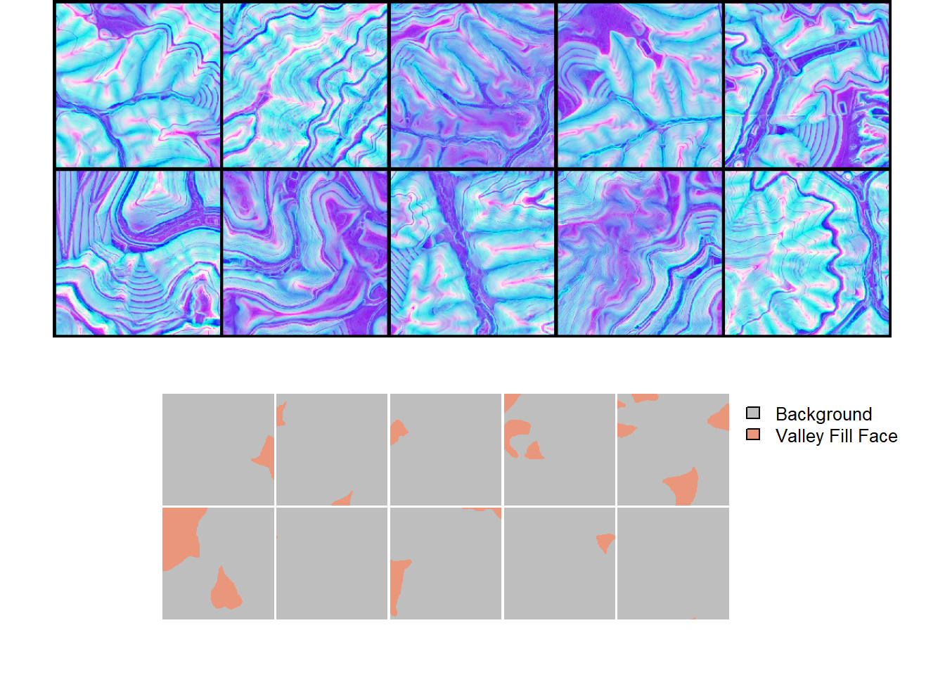
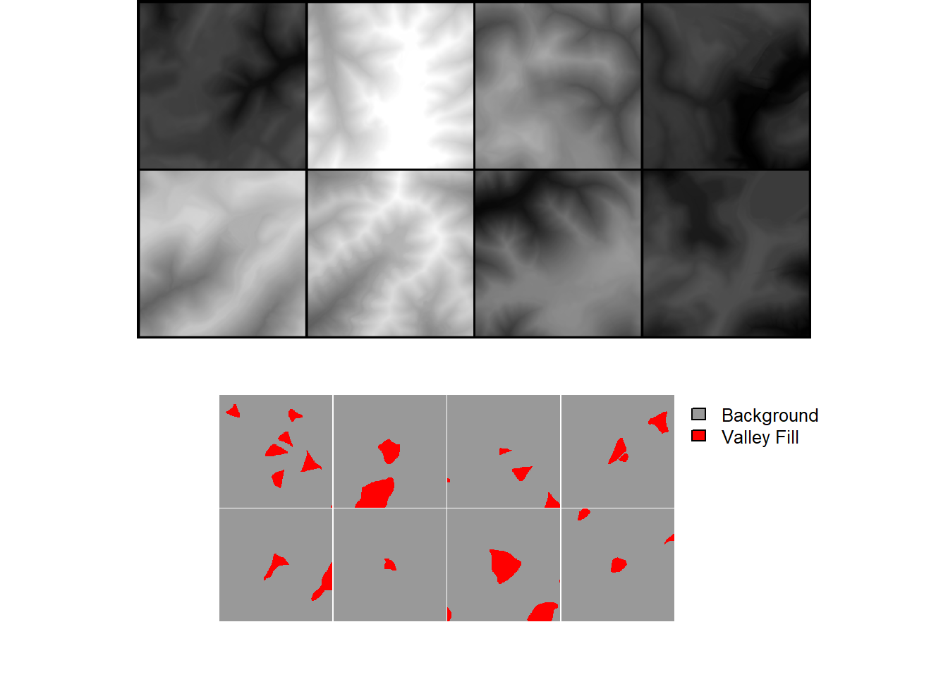
drop_last = FALSE)As noted in the prior chapter, we recommend checking your data with geodl’s utility functions prior to training a model. We view a mini-batch of chips and associated masks using viewBatch(). We also obtain summary information for all three data partitions using describeBatch(). The predictor variables and masks look correct. The mini-batch size (10), number of bands (3), and spatial dimension sizes (512x512) are as expected. The class codes are 1 and 2, also as expected. In short, everything looks good.
Within viewBatch(), we set cCodes to c(1,2) as opposed to c(0,1) since the dataset subclasses were configured to add 1 to each class code.
viewBatch(dataLoader=trainDL,
          nCols = 5,
          r = 1,
          g = 2,
          b = 3,
          cCodes=c(1, 2),
          cNames=c("Background", "Valley Fill Face"),
          cColors=c("gray", "darksalmon")
)
trainStats <- describeBatch(trainDL,
                            zeroStart=FALSE)
valStats <- describeBatch(valDL,
                          zeroStart=FALSE)
testStats <- describeBatch(testDL,
zeroStart=FALSE)trainStats$batchSize
[1] 10
$imageDataType
[1] "Float"
$maskDataType
[1] "Long"
$imageShape
[1] "10" "3" "512" "512"
$maskShape
[1] "10" "1" "512" "512"
$bndMns
[1] 0.5020081 0.4720880 0.5000184
$bandSDs
[1] 0.17379957 0.14551426 0.01439747
$maskCount
[1] 2446092 175348
$minIndex
[1] 1
$maxIndex
[1] 2valStats$batchSize
[1] 10
$imageDataType
[1] "Float"
$maskDataType
[1] "Long"
$imageShape
[1] "10" "3" "512" "512"
$maskShape
[1] "10" "1" "512" "512"
$bndMns
[1] 0.5023526 0.4569009 0.5000239
$bandSDs
[1] 0.15027517 0.13255997 0.01142568
$maskCount
[1] 2600276 21164
$minIndex
[1] 1
$maxIndex
[1] 2testStats$batchSize
[1] 10
$imageDataType
[1] "Float"
$maskDataType
[1] "Long"
$imageShape
[1] "10" "3" "512" "512"
$maskShape
[1] "10" "1" "512" "512"
$bndMns
[1] 0.5006625 0.4646924 0.5000082
$bandSDs
[1] 0.17750140 0.14047340 0.01387529
$maskCount
[1] 2610809 10631
$minIndex
[1] 1
$maxIndex
[1] 216.3.3 Training Loop
Now that are datasets and dataloaders have been configured and instantiated and we have performed checks, we are ready to train the model. We will implement a UNet architecture via defineUNet(). We configure the unified focal loss framework to use a focal Tversky loss. Two classes are being differentiated. lambda is set to 0 so that only the region-based loss is used. delta is set to 0.6, which results in more weight being applied to false negative (FN) errors. Since gamma is < 1, more weight will be placed on difficult samples. We also change the class weighting in the region-based loss so that the positive case has a higher weight (0.7) than the background case (0.3). zeroStart is set to FALSE since the class codes start at 1 as opposed to 0.
We use the AdamW optimizer with a learning rate of 0.001. We calculate four assessment metrics: overall accuracy, f1-score, recall, and precision. The last three metrics are calculated for only the positive case, as is common for a binary classification task, by setting clsWghts to c(0,1).
The UNet architecture is is configured to accept 3 predictor variables and differentiate 2 classes. We also make use of the leaky rectified linear unit (ReLU) activation function and residual connections. We define the number of output feature maps for each encoder block, the bottleneck, each decoder block, and all branches of the ASPP module. We also specify dilation rates to use within the ASPP module.
We train the model for a total of 25 epochs, log the training and validation losses and assessment metrics to a CSV file, and save the state dictionary after each epoch. luz takes care of implementing GPU-based acceleration.
If you choose to run the training loop, it will take several hours to execute. We have provided a trained model in the data folder for the chapter if you would like to execute the following code without training a new model. The file is named “vfillModel.pt.” We have also included the training logs: “vfillTrainLogs.csv”. If you want to load our model, the UNet must use the exact same configuration as we have specified below.
fitted <- defineUNet |>
  luz::setup(
    loss = defineUnifiedFocalLoss(nCls=2,
                                  lambda=0,
                                  gamma=.7,
                                  delta=0.6,
                                  smooth = 1e-8,
                                  zeroStart=FALSE,
                                  clsWghtsDist=1,
                                  clsWghtsReg=c(0.3, 0.7),
                                  useLogCosH =FALSE,
                                  device="cuda"),
    optimizer = optim_adamw,
    metrics = list(
      luz_metric_overall_accuracy(nCls=2,
                                  smooth=1,
                                  mode = "multiclass",
                                  zeroStart= FALSE),
      luz_metric_f1score(nCls=2,
                         smooth=1,
                         mode = "multiclass",
                         zeroStart= FALSE,
                         clsWghts=c(0,1)),
      luz_metric_recall(nCls=2,
                        smooth=1,
                        mode = "multiclass",
                        zeroStart= FALSE,
                        clsWghts=c(0,1)),
      luz_metric_precision(nCls=2,
                           smooth=1,
                           mode = "multiclass",
                           zeroStart= FALSE,
                           clsWghts=c(0,1))
    )
  ) |>
  set_hparams(inChn = 3,
              nCls = 2,
              actFunc = "lrelu",
              useAttn = FALSE,
              useSE = FALSE,
              useRes = TRUE,
              useASPP = TRUE,
              useDS = FALSE,
              enChn = c(16,32,64,128),
              dcChn = c(128,64,32,16),
              btnChn = 256,
              dilRates=c(1,2,4,8,16),
              dilChn=c(128,128,128,128),
              negative_slope = 0.01) |>
  set_opt_hparams(lr = 1e-3) |>
  fit(data = trainDL,
      epochs = 25,
      valid_data = valDL,
      callbacks = list(luz_callback_csv_logger("D:/vfillDLMini/vfillDLMini/vfillLogs.csv"),
                       callback_save_model_state_dict(save_dir = "D:/vfillDLMini/vfillDLMini/", prefix = "epoch")),
      accelerator = accelerator(device_placement = TRUE,
                                cpu = FALSE,
                                cuda_index = torch::cuda_current_device()),
      verbose=TRUE)
16.3.4 Model Validation
We now load in our saved logs and plot the trends in the training and validation assessment metrics over the training epochs. We have chosen to use the result after epoch 20 since it provided a good F1-score.
#Read in saved metrics
allMets <- read_csv(str_glue('gslrData/chpt16/data/vfillTrainLogs.csv'))

#Graph losses
ggplot(allMets, aes(x=epoch, y=loss, color=set))+
  geom_line(lwd=1)+
  labs(x="Epoch", y="Loss", color="Set")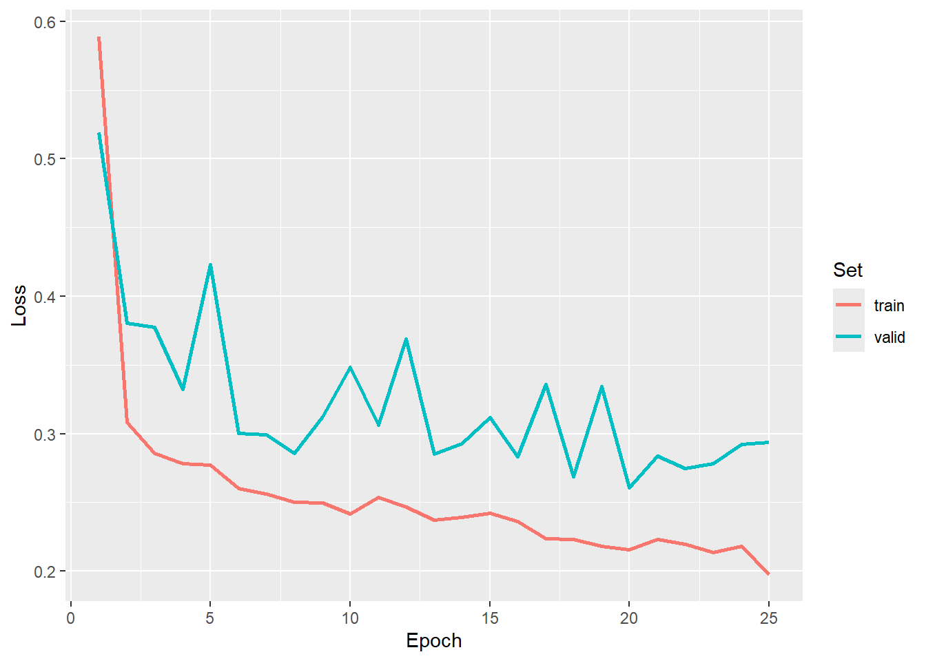
#Graph F1-score
ggplot(allMets, aes(x=epoch, y=f1score, color=set))+
  geom_line(lwd=1)+
  labs(x="Epoch", y="F1-Score", color="Set")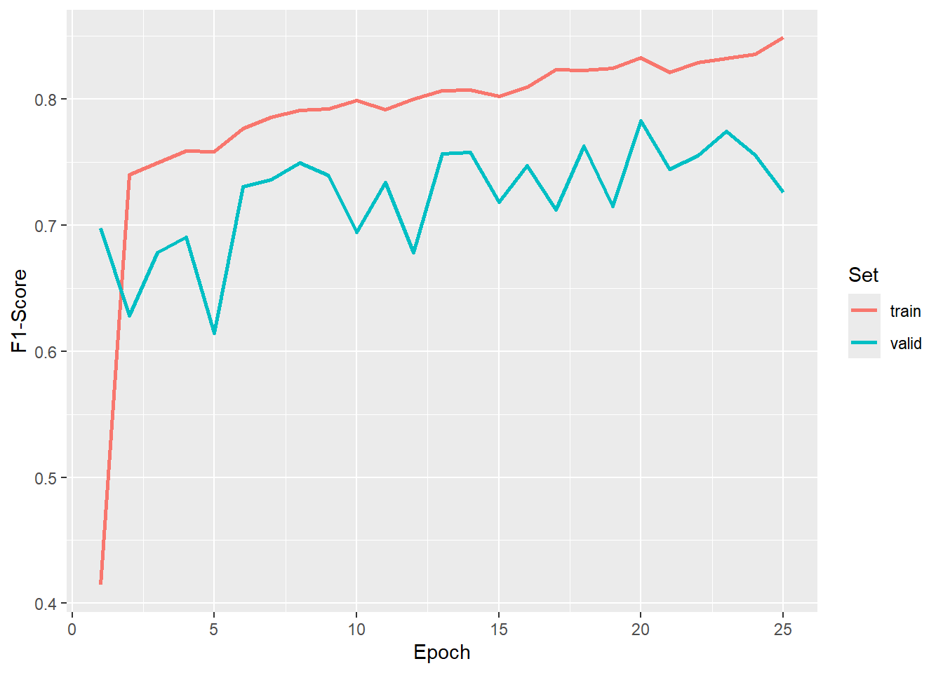
#Graph recall
ggplot(allMets, aes(x=epoch, y=recall, color=set))+
  geom_line(lwd=1)+
  labs(x="Epoch", y="Recall", color="Set")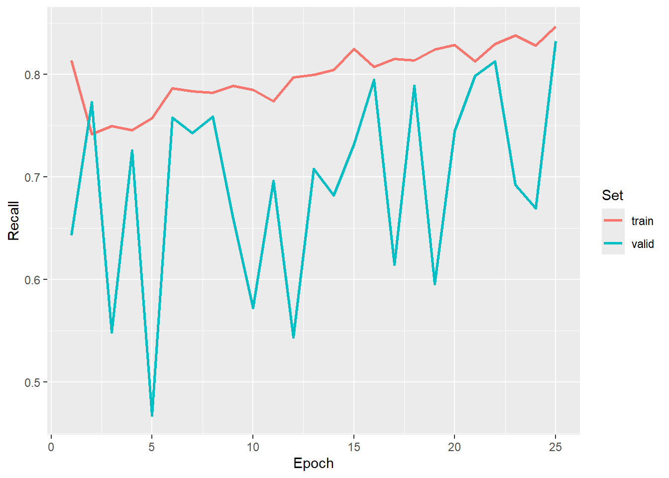
#Graph precision
ggplot(allMets, aes(x=epoch, y=precision, color=set))+
  geom_line(lwd=1)+
  labs(x="Epoch", y="Precision", color="Set")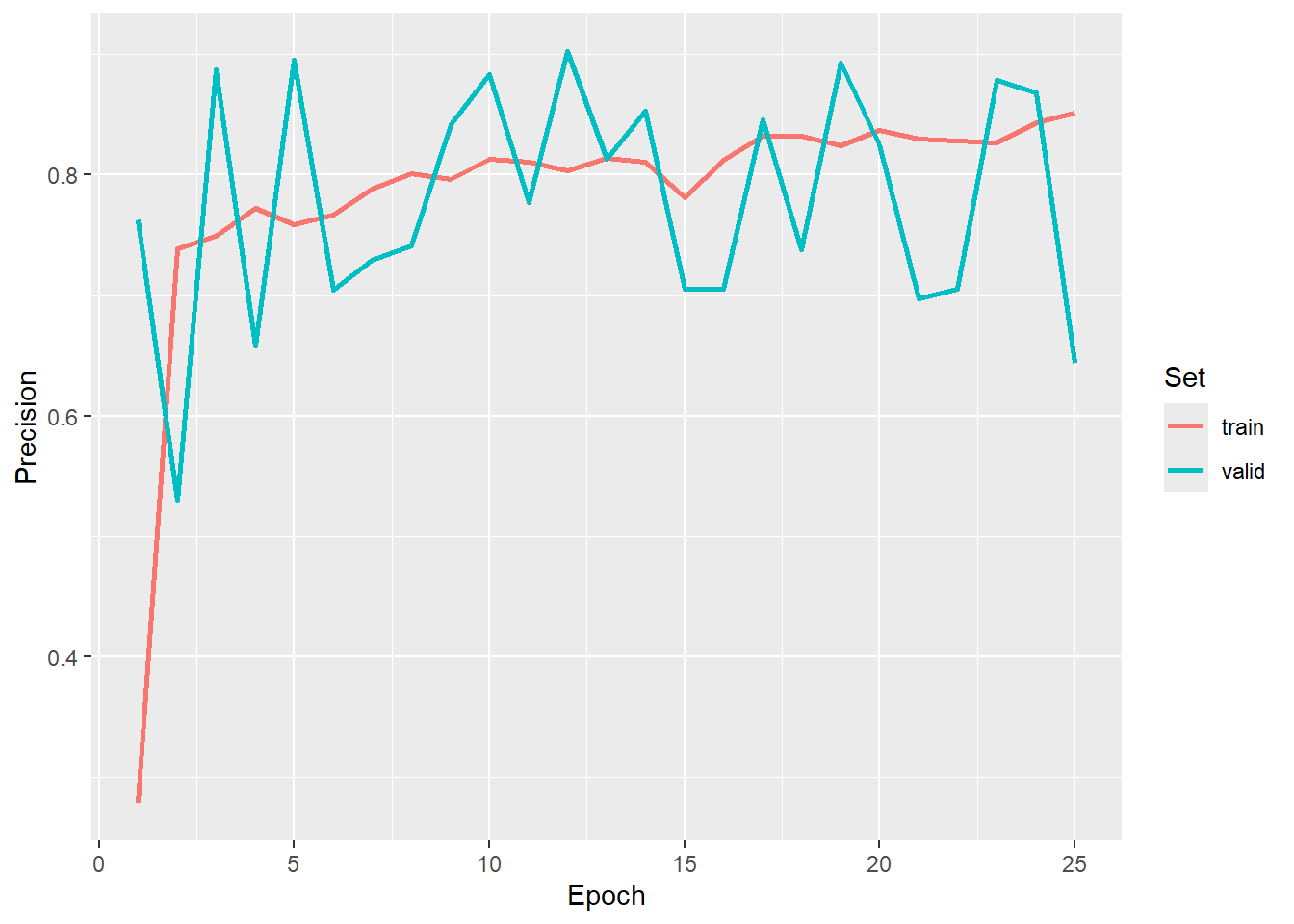
In order to use our saved model, we re-instantiate an instance of the model with the exact same configuration as the version that was trained. We next load the saved state dictionary into the the model and place it in evaluation mode.
We recommend moving the model to the GPU using $to(device="cuda") to speed up inference.
When loading a saved state dictionary, it is necessary to instantiate a model that has the exact same configuration as the model that was trained so that all of the parameters can be matched.
When the model is used for validation or to make predictions, it must be placed in evaluation mode so that it behaves correctly. Although geodl’s prediction and assessment functions do this internally, we recommend explicitly placing the model in evaluation mode using $eval() after loading a saved state from disk.
newModel <- defineUNet(inChn = 3,
                       nCls = 2,
                       actFunc = "lrelu",
                       useAttn = FALSE,
                       useSE = FALSE,
                       useRes = TRUE,
                       useASPP = TRUE,
                       useDS = FALSE,
                       enChn = c(16,32,64,128),
                       dcChn = c(128,64,32,16),
                       btnChn = 256,
                       dilRates=c(1,2,4,8,16),
                       dilChn=c(128,128,128,128),
                       negative_slope = 0.01)$to(device="cuda")

newModel$load_state_dict(torch_load("gslrData/chpt16/data/vfillModel.pt"))
newModel$eval()
The viewBatchPreds() function plots a mini-batch of predictor variable chips, reference masks, and prediction masks and is meant to provide a visual assessment of the prediction results for a subset of image chips. The assessDL() function generates a variety of assessment metrics using all mini-batches generated by a dataloader. Note that this can be slow due to the large volume of computations being performed. In this example, we set multiclass to FALSE to obtain binary classification assessment metrics as opposed to multiclass metrics. Practically, this means that the F1-score, recall, and precision metrics only consider the positive case. Also, the negative predictive value (NPV) and specificity are calculate for the negative case.
viewBatchPreds(dataLoader=testDL,
               model=newModel,
               mode="multiclass",
               nCols =4,
               r = 1,
               g = 2,
               b = 3,
               cCodes=c(1,2),
               cNames=c("Background", "Valley Fill Face"),
               cColors=c("gray", "darksalmon"),
               useCUDA=TRUE,
               probs=FALSE,
               usedDS=FALSE)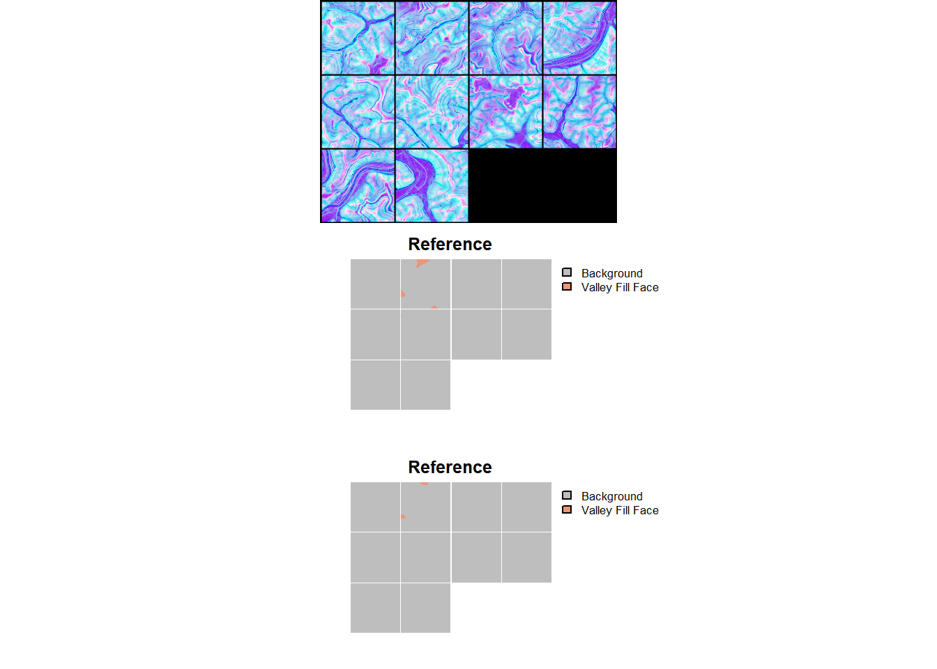
metricsOut <- assessDL(dl=testDL,
                       model=newModel,
                       batchSize=8,
                       size=512,
                       nCls=2,
                       multiclass=FALSE,
                       cCodes=c(1,2),
                       cNames=c("Background", "Valley Fill Face"),
                       usedDS=FALSE,
                       useCUDA=TRUE,
                       decimals=4)

print(metricsOut)
$Classes
[1] "Background" "Valley Fill Face"
$referenceCounts
Negative Positive
102524295 2333305
$predictionCounts
Negative Positive
103334045 1523555
$ConfusionMatrix
Reference
Predicted Negative Positive
Negative 102273149 1060896
Positive 251146 1272409
$Mets
OA Recall Precision Specificity NPV F1Score
Valley Fill Face 0.9875 0.5453 0.8352 0.9976 0.9897 0.659816.3.5 Spatial Prediction
In the final step in the workflow, we use our trained and validated model to predict to a new spatial extent. This is accomplished using the predictSpatial() function. To obtain a “hard” classification, we set predType to "class". We use a stride in both the x and y directions that is smaller than the chip size to process the prediction using overlap. We also remove the outer 50 rows and columns of predictions from all non-edge chips so that only the center of chips are used in the final prediction when possible. The prediction is performed using a GPU to speed up the computation.
The new data and the resulting prediction have been provided in the data folder for the chapter. The input data are named “dtmStk.tif” while the example prediction is named “dtmPred2.tif”
predCls <- predictSpatial(imgIn=str_glue("gslrData/chpt16/data/dtmStk.tif"),
                          model=newModel,
                          predOut=str_glue("gslrData/chpt16/data/dtmPred2.tif"),
                          mode="multiclass",
                          predType="class",
                          useCUDA=TRUE,
                          nCls=2,
                          chpSize=512,
                          stride_x=256,
                          stride_y=256,
                          crop=50,
                          nChn=3,
                          normalize=FALSE,
                          rescaleFactor=1,
                          usedDS=FALSE)
Once the prediction is generated, it can be visualized using tmap.
16.4 Workflow 2: Valley Fills (Dynamic)
We will now explore the same task as that explored in Workflow 1. However, we will now make use of dynamic chip generation and the TerrainSeg framework implemented by geodl. This requires working with the original input DTM data and vector-based valley fill face examples as opposed to image chips, raster-based masks, and derived LSPs.
As normal, we begin by loading the required libraries and setting our working directory.
It is not necessary for us to reload libraries here. We are simply doing so in order to make each workflow stand-alone.
fldPth2 <- "D:/22318522/vfillDL/vfillDL/"16.4.1 Preparation
To use the dynamic chips workflow, example vector data must have a “code” column that assigns a unique integer to each class being differentiated and also a “class” column that names the class. Our example data do contain a “code” column but they lack a “class” column; as a result, we use dplyr to add this needed column. We then save the vector data back to disk with st_write().
trainExt <- st_read(str_glue("{fldPth2}extents/training.shp"), quiet=TRUE)
val1Ext <- st_read(str_glue("{fldPth2}extents/validation1.shp"), quiet=TRUE)
val2Ext <- st_read(str_glue("{fldPth2}extents/validation2.shp"), quiet=TRUE)
ky1Ext <- st_read(str_glue("{fldPth2}extents/testingKY1.shp"), quiet=TRUE)
ky2Ext <- st_read(str_glue("{fldPth2}extents/testingKY2.shp"), quiet=TRUE)
va1Ext <- st_read(str_glue("{fldPth2}extents/testingVA1.shp"), quiet=TRUE)
trainV <- st_read(str_glue("{fldPth2}vectors/training.shp"), quiet=TRUE) |>
mutate(class = "vfill") |>
st_write(str_glue("{fldPth2}vectors/trainingb.shp"),
append=FALSE)
val1V <- st_read(str_glue("{fldPth2}vectors/validation.shp"), quiet=TRUE) |>
mutate(class = "vfill") |>
st_write(str_glue("{fldPth2}vectors/validationb.shp"),
append=FALSE)
val2V <- st_read(str_glue("{fldPth2}vectors/validation2.shp"), quiet=TRUE) |>
mutate(class = "vfill") |>
st_write(str_glue("{fldPth2}vectors/validation2b.shp"),
append=FALSE)
ky1V <- st_read(str_glue("{fldPth2}vectors/testingKY1.shp"), quiet=TRUE) |>
mutate(class = "vfill") |>
st_write(str_glue("{fldPth2}vectors/testingKY1b.shp"),
append=FALSE)
ky2V <- st_read(str_glue("{fldPth2}vectors/testingKY2.shp"), quiet=TRUE) |>
mutate(class = "vfill") |>
st_write(str_glue("{fldPth2}vectors/testingKY2b.shp"),
append=FALSE)
va1V <- st_read(str_glue("{fldPth2}vectors/testingVA1.shp"), quiet=TRUE) |>
mutate(class = "vfill") |>
st_write(str_glue("{fldPth2}vectors/testingVA1b.shp"),
append=FALSE)Before moving on, we visualize the extents and vector reference data. We bind all the extents into a single object then do the same for the example features. The example features are then converted to points using st_centroid(). This is just for display purposes. The data consist of six separate study areas: three in southern West Virginia, two in eastern Kentucky, and one in southwestern Virginia.
allExtents <- bind_rows(trainExt,
                        val1Ext,
                        val2Ext,
                        ky1Ext,
                        ky2Ext,
                        va1Ext)

allFeatures <- bind_rows(trainV,
                         val1V,
                         val2V,
                         ky1V,
                         ky2V,
                         va1V)

allFeaturesPnts <- st_centroid(allFeatures)
osm <- read_osm(st_bbox(st_buffer(allExtents, 3000)))
tm_shape(osm)+
tm_rgb()+
tm_shape(allExtents)+
tm_borders(col="black", lwd=2)+
tm_shape(allFeaturesPnts)+
tm_bubbles(fill="red", size=.5)+
tm_compass(position=c("left", "bottom"))+
tm_scalebar(position=c("left", "bottom"))
16.4.2 Datasets and Dataloaders
We now work through the the steps required to implement the dynamic chips workflow. We first use makeDynamicChipsSF() to generate sf objects for each extent. This requires defining the boundary, vector features, and associated DTM for each region. We have also chosen to generate random background point locations to generate additional background-only chips. The resulting data are also shuffled to potentially reduce spatial autocorrelation. We use a minimum distance of 100 m between the random background point locations and the presence point locations.
trainDC <- makeDynamicChipsSF(
  featPth = str_glue("{fldPth2}vectors/"),
  featName = "trainingb.shp",
  extentPth = str_glue("{fldPth2}extents/"),
  extentName = "training.shp",
  extentCrop = 0,
  imgPth <- str_glue("{fldPth2}dems/"),
  imgName <- "train_dem.img",
  doBackground = FALSE,
  backgroundCnt = 500,
  backgroundDist = 100,
  useSeed = TRUE,
  seed = 42,
  doShuffle = TRUE
)

val1DC <- makeDynamicChipsSF(
  featPth = str_glue("{fldPth2}vectors/"),
  featName = "validationb.shp",
  extentPth = str_glue("{fldPth2}extents/"),
  extentName = "validation1.shp",
  extentCrop = 200,
  imgPth <- str_glue("{fldPth2}dems/"),
  imgName <- "val_dem.tif",
  doBackground = TRUE,
  backgroundCnt = 200,
  backgroundDist = 100,
  useSeed = TRUE,
  seed = 42,
  doShuffle = TRUE
)

val2DC <- makeDynamicChipsSF(
  featPth = str_glue("{fldPth2}vectors/"),
  featName = "validation2b.shp",
  extentPth = str_glue("{fldPth2}extents/"),
  extentName = "validation2.shp",
  extentCrop = 200,
  imgPth <- str_glue("{fldPth2}dems/"),
  imgName <- "test_dem.tif",
  doBackground = TRUE,
  backgroundCnt = 200,
  backgroundDist = 100,
  useSeed = TRUE,
  seed = 42,
  doShuffle = TRUE
)

ky1DC <- makeDynamicChipsSF(
  featPth = str_glue("{fldPth2}vectors/"),
  featName = "testingKY1b.shp",
  extentPth = str_glue("{fldPth2}extents/"),
  extentName = "testingKY1.shp",
  extentCrop = 200,
  imgPth <- str_glue("{fldPth2}dems/"),
  imgName <- "ky1_dem.tif",
  doBackground = TRUE,
  backgroundCnt = 100,
  backgroundDist = 100,
  useSeed = TRUE,
  seed = 42,
  doShuffle = TRUE
)

ky2DC <- makeDynamicChipsSF(
  featPth = str_glue("{fldPth2}vectors/"),
  featName = "testingKY2b.shp",
  extentPth = str_glue("{fldPth2}extents/"),
  extentName = "testingKY2.shp",
  extentCrop = 200,
  imgPth <- str_glue("{fldPth2}dems/"),
  imgName <- "ky_2_dem.tif",
  doBackground = TRUE,
  backgroundCnt = 100,
  backgroundDist = 100,
  useSeed = TRUE,
  seed = 42,
  doShuffle = TRUE
)

va1DC <- makeDynamicChipsSF(
  featPth = str_glue("{fldPth2}vectors/"),
  featName = "testingVA1b.shp",
  extentPth = str_glue("{fldPth2}extents/"),
  extentName = "testingVA1.shp",
  extentCrop = 200,
  imgPth <- str_glue("{fldPth2}dems/"),
  imgName <- "va1_dem.tif",
  doBackground = TRUE,
  backgroundCnt = 100,
  backgroundDist = 100,
  useSeed = TRUE,
  seed = 42,
  doShuffle = TRUE
)
Next, we bind the data frames to generate three partitions: training, validation, and test. The large extent in West Virginia is used for training while the other two extents in West Virginia are used for validation during the training process. The extents in Kentucky and Virginia are used to assess the final model as a test set. Since the result is an sf object, which behaves as a data frame with associated spatial information, this can be accomplished using bind_rows().
If desired, the results could be saved to disk as geospatial vector files.
We now check the chips using checkDynamicChips(). This is to make sure that the generated chips do not (1) contain NA cells and (2) do not have incorrect dimensions or shapes. Issues can arise due to chips occurring near the edge of extents. Note that such issues can be partially avoided by using an extent smaller than the area covered by the raster-based predictor variables. We specifically remove any samples that contain NA cells in either the chips or masks and/or that have a number of rows and/or columns not equal to that desired (i.e., 512x512).
cSize = 640

trainDC <- trainDC |>
  checkDynamicChips(chipSize=cSize,
                    cellSize=2,
                    doJitter=FALSE) |>
  filter(cCntImg == cSize &
           rCntImg == cSize &
           cCntMsk == cSize &
           rCntMsk == cSize &
           naCntImg == 0 &
           naCntMsk == 0)


testDC <- testDC |>
  checkDynamicChips(chipSize=cSize,
                    cellSize=2,
                    doJitter=FALSE) |>
  filter(cCntImg == cSize &
           rCntImg == cSize &
           cCntMsk == cSize &
           rCntMsk == cSize &
           naCntImg == 0 &
           naCntMsk == 0)


valDC <- valDC |>
  checkDynamicChips(chipSize=cSize,
                    cellSize=2,
                    doJitter=FALSE) |>
  filter(cCntImg == cSize &
           rCntImg == cSize &
           cCntMsk == cSize &
           rCntMsk == cSize &
           naCntImg == 0 &
           naCntMsk == 0)
Now that the chips have been checked, we can instantiate DataSet instances using defineDynamicSegDataSet(). This works the same as defineSegDataSet() other than that the input must be generated by defineDynamicChipsSF() and the size of the chips must be specified. We can still incorporate random augmentations, normalization, and re-scaling as desired. For the training data, we apply some random augmentations and add 1 to the mask values to obtain codes of 1 and 2. For the other two partitions, random augmentations are not applied, but we still add 1 to the class codes.
Random noise or jitter can be added to the center coordinates for each chip so that the chip is not directly centered over the centroid of a reference feature. This can potentially add more variability to the dataset. We are not making use of this option here. If you do use this option, the same settings should be used with checkDynamicChips().
trainDS <- defineDynmamicSegDataSet(chipsSF=trainDC,
                                    chipSize=cSize,
                                    cellSize=2,
                                    doJitter=FALSE,
                                    normalize = FALSE,
                                    rescaleFactor = 1,
                                    mskRescale=1,
                                    mskAdd=1,
                                    doAugs = TRUE,
                                    maxAugs = 3,
                                    probVFlip = .3,
                                    probHFlip = .3,
                                    probRotate= .3)

valDS <- defineDynmamicSegDataSet(chipsSF=valDC,
                                    chipSize=cSize,
                                    cellSize=2,
                                    doJitter=FALSE,
                                    normalize = FALSE,
                                    rescaleFactor = 1,
                                    mskRescale=1,
                                    mskAdd=1,
                                    doAugs = FALSE)

testDS <- defineDynmamicSegDataSet(chipsSF=testDC,
                                    chipSize=cSize,
                                    cellSize=2,
                                    doJitter=FALSE,
                                    normalize = FALSE,
                                    rescaleFactor = 1,
                                    mskRescale=1,
                                    mskAdd=1,
                                    doAugs = FALSE)
We next instantiate the three torch dataloaders. We use a smaller mini-batch size in this workflow than in Workflow 1 since the model is larger and more complex. Again, you may need to change the mini-batch size depending on your available hardware. We shuffle the training set but not the validation or test set. For all partitions, we drop the last mini-batch since it may be incomplete (i.e., the number of chips is not evenly divisible by the mini-batch size).
trainDL <- torch::dataloader(trainDS,
                             batch_size=8,
                             shuffle=TRUE,
                             drop_last = TRUE)

testDL <- torch::dataloader(testDS,
                            batch_size=8,
                            shuffle=FALSE,
                            drop_last = TRUE)

valDL <- torch::dataloader(valDS,
                           batch_size=8,
                           shuffle=FALSE,
                           drop_last = TRUE)
As checks, we print the length of each data loader and view a batch of chips from each partition.
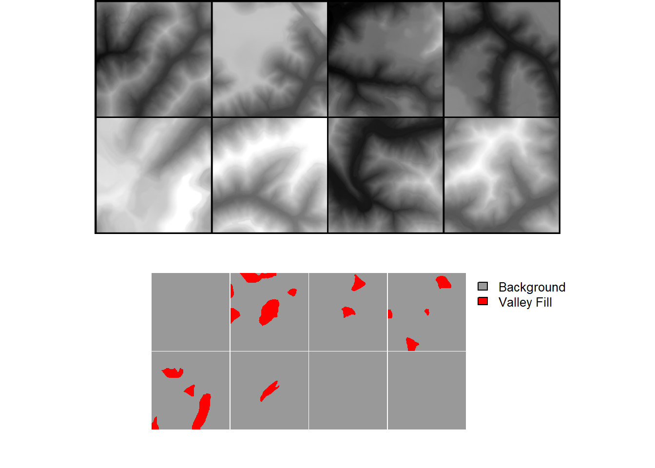
viewBatch(dataLoader=trainDL,
          nCols = 4,
          r = 1,
          g = 1,
          b = 1,
          cCodes = c(1,2),
          cNames=c("Background", "Valley Fill"),
          cColors=c("gray60", "red")
)
16.4.3 Training Loop
The training loop set up is very similar to Workflow 1. We are using the same loss function (focal Tversky loss), assessment metrics (overall accuracy, F1-score, precision, and recall), and optimization algorithm (AdamW). For the loss and assessment metrics we have now implemented a crop factor so that edge rows and columns do not contribute to the loss or assessment metric calculations. The assessment metrics have been configured for a binary classification where only the positive case is considered using class weights of c(0,1).
For the model, we are using defineTerrainSeg(), and the trainable component is the UNet3+ archtiecture with default settings other than using leaky ReLU activation. For the LSP calculations, we use an inner radius of 2 cells and an outer radius of 10 cells for the local TPI calculation. For the hillslope-scale TPI calculation, we use a radius of 50 meters. We use a smoothing radius of 11 cells for the curvature calculations. Lastly, we do not use Gaussian Pyramids. As a result, a total of 6 LSPs are provided to the trainable UNet3+ model.
Between the LSP module and trainable UNet3+ model, we apply a crop of 64 rows and columns of cells. Since the input data have an input size of 640x640, this means that the input to the UNet3+ model will have a spatial size of 512x512. We recommend using an input size and crop combination that results in an input size to the trainable component of the model of 1024x1024, 512x512, or 256x256. This will allow for appropriate tensor sizes throughout the down scaling processes in the semantic segmentation component of the model.
As with Workflow 1, we save the model logs and the state dictionary at the end of each epoch. luz handles GPU-based acceleration.
This took several hours to run on our machine. As with Workflow 1, we provided output files. The trained model is provided as “vfillDynamicModel.pt” while the log is provided as “vfillDynamicTrainLog.csv”.
fitted <- defineTerrainSeg |>
  luz::setup(
    loss = defineUnifiedFocalLoss(nCls=2,
                                  cropFactorMsk = 64,
                                  lambda=0,
                                  gamma=.7,
                                  delta=0.6,
                                  smooth = 1e-8,
                                  zeroStart=FALSE,
                                  clsWghtsDist=1,
                                  clsWghtsReg=c(0.3, 0.7),
                                  useLogCosH =FALSE,
                                  device="cuda"),
    optimizer = optim_adamw,
    metrics = list(
      luz_metric_overall_accuracy(nCls=2,
                                  cropFactorMsk=64,
                                  smooth=1,
                                  mode = "multiclass",
                                  zeroStart= FALSE),
      luz_metric_f1score(nCls=2,
                         cropFactorMsk=64,
                         smooth=1,
                         mode = "multiclass",
                         zeroStart= FALSE,
                         clsWghts=c(0,1)),
      luz_metric_recall(nCls=2,
                        cropFactorMsk=64,
                        smooth=1,
                        mode = "multiclass",
                        zeroStart= FALSE,
                        clsWghts=c(0,1)),
      luz_metric_precision(nCls=2,
                           cropFactorMsk=64,
                           smooth=1,
                           mode = "multiclass",
                           zeroStart= FALSE,
                           clsWghts=c(0,1))
    )
  ) |>
  set_hparams(segModel="UNet3p",
              nCls = 2,
              cellSize = 2,
              spatDim=640,
              tCrop = 64,
              doGP = FALSE,
              innerRadius = 2,
              outerRadius = 10,
              hsRadius = 50,
              smoothRadius = 11,
              actFunc="lrelu",
              negative_slope = 0.01) |>
  set_opt_hparams(lr = 1e-3,
                  ) |>
  fit(data = trainDL,
      epochs = 25,
      valid_data = valDL,
      callbacks = list(luz_callback_csv_logger(str_glue("{fldPth2}experiments/vfillLogs.csv")),
                       callback_save_model_state_dict(save_dir =str_glue("{fldPth2}experiments/"),
                                                      prefix = "epoch")),
      accelerator = accelerator(device_placement = TRUE,
                                cpu = FALSE,
                                cuda_index = torch::cuda_current_device()),
      verbose=TRUE)
16.4.4 Model Validation
Once the workflow is trained, we explore the training logs. Based on the results, we selected the model state after epoch 23 as the final model. This is the model that has been provided in the data folder for the chapter.
#Read in saved metrics
allMets <- read_csv("gslrData/chpt16/data/vfillDynamicTrainLogs.csv")

#Graph losses
ggplot(allMets, aes(x=epoch, y=loss, color=set))+
  geom_line(lwd=1)+
  labs(x="Epoch", y="Loss", color="Set")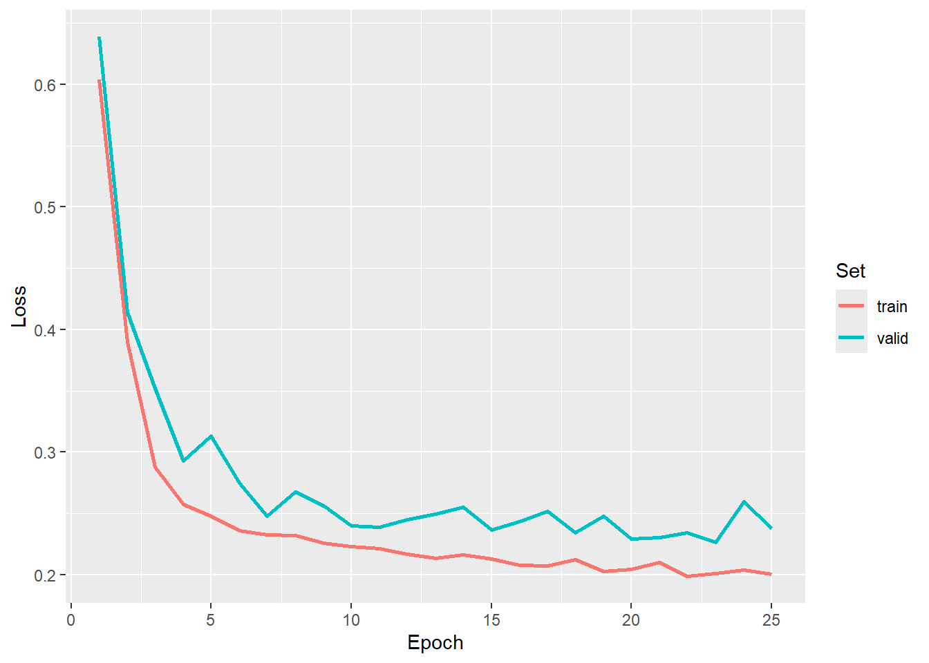
#Graph F1-score
ggplot(allMets, aes(x=epoch, y=f1score, color=set))+
  geom_line(lwd=1)+
  labs(x="Epoch", y="F1-Score", color="Set")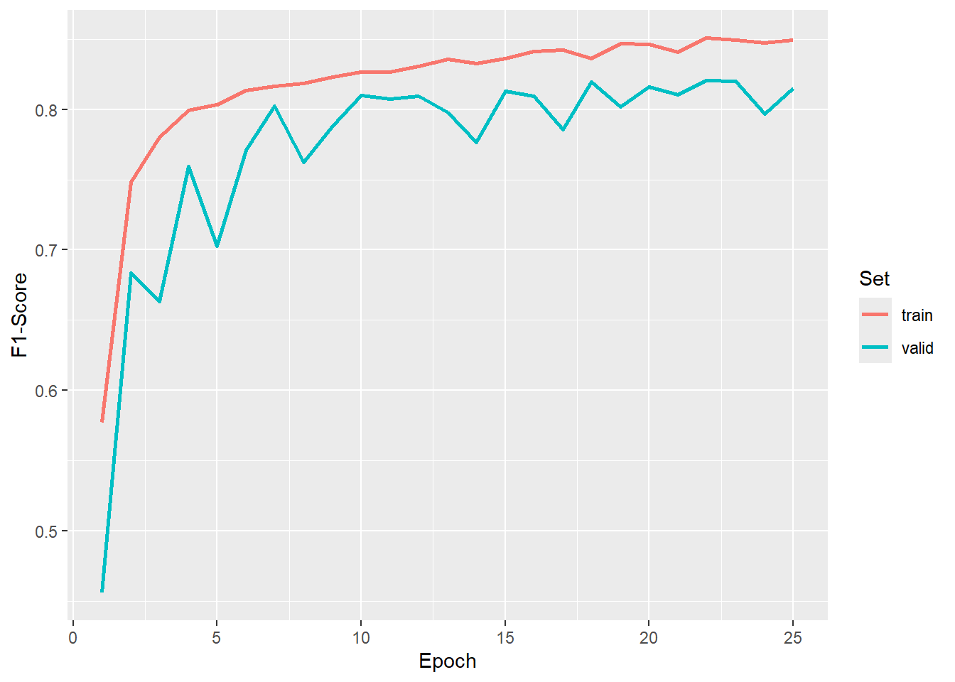
#Graph recall
ggplot(allMets, aes(x=epoch, y=recall, color=set))+
  geom_line(lwd=1)+
  labs(x="Epoch", y="Recall", color="Set")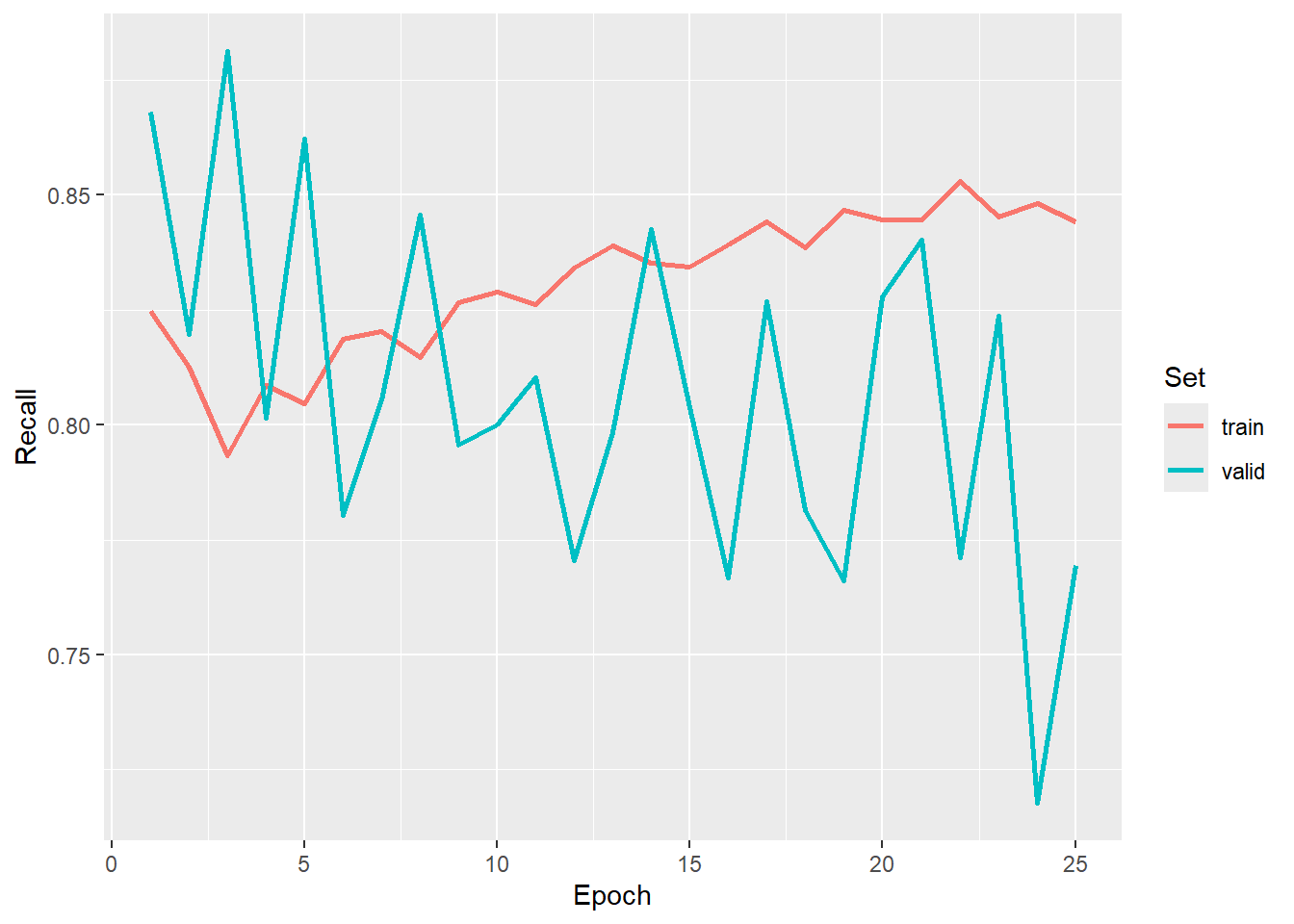
#Graph precision
ggplot(allMets, aes(x=epoch, y=precision, color=set))+
  geom_line(lwd=1)+
  labs(x="Epoch", y="Precision", color="Set")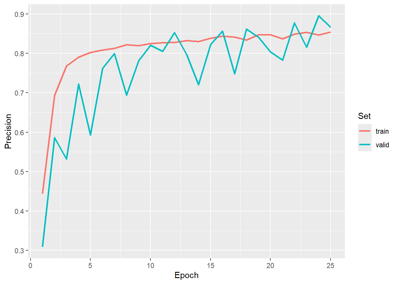
The model is re-instantiated, the state dictionary is loaded, and the model is placed in evaluation mode. Again, it is important that the instantiated model is identical to the model that was trained so that the trainable parameters can be correctly matched and loaded from the saved state dicationary.
newModel <- defineTerrainSeg(segModel="UNet3p",
nCls = 2,
cellSize = 2,
spatDim=640,
tCrop = 64,
doGP = FALSE,
innerRadius = 2,
outerRadius = 10,
hsRadius = 50,
smoothRadius = 11,
actFunc="lrelu",
negative_slope = 0.01)$to(device="cuda")
newModel$load_state_dict(torch_load(str_glue("gslrData/chpt16/data/vfillDynamicModel.pt")))
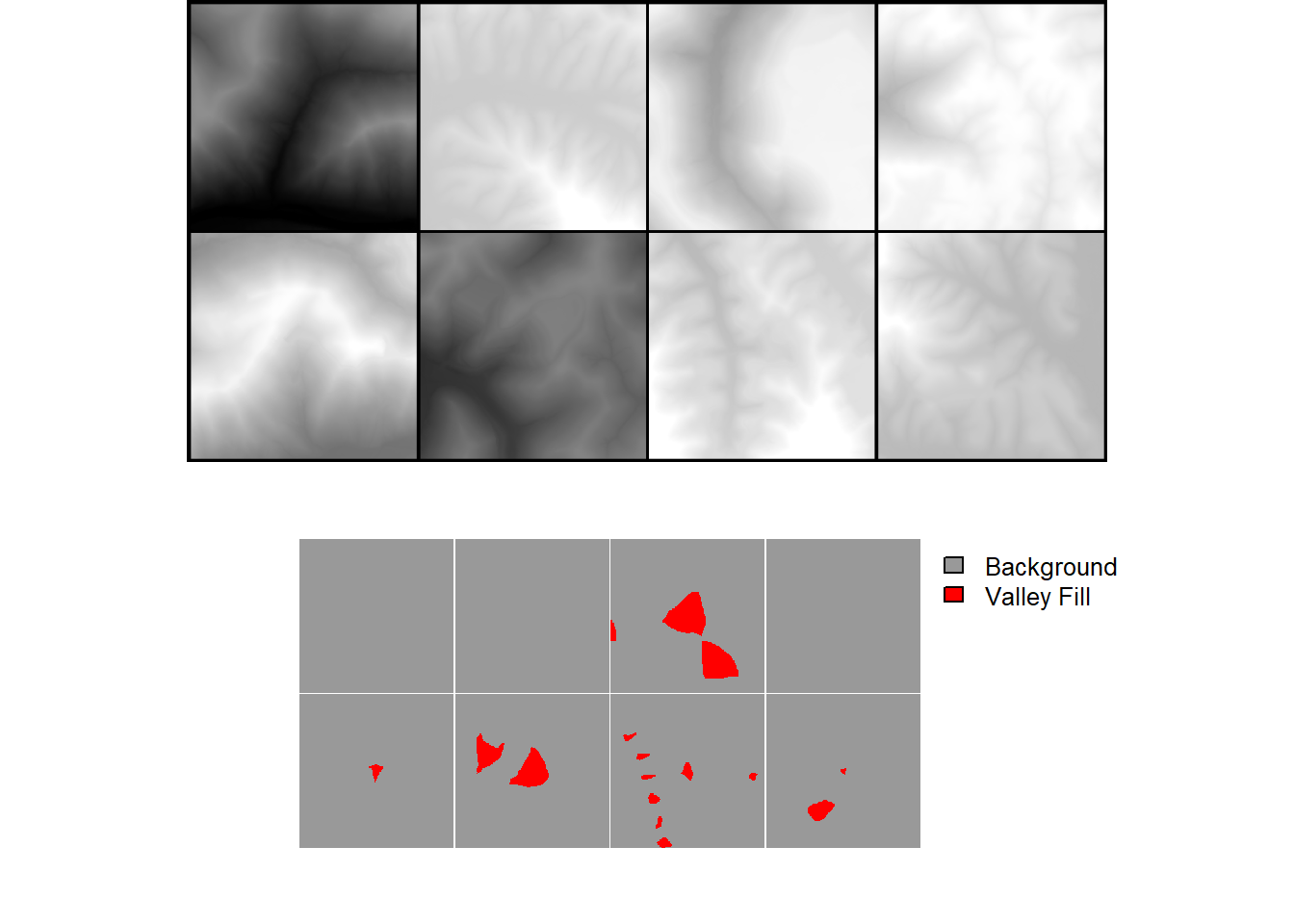
newModel$eval()As with Workflow 1, a mini-batch of predictions can be visualized using viewBatchPreds(), and the model can be validated using the test data and assessDL() function.
viewBatchPreds(dataLoader=testDL,
               model=newModel,
               mode="multiclass",
               nCols =4,
               padding=20,
               r = 1,
               g = 1,
               b = 1,
               cCodes=c(1,2),
               cNames=c("Background", "Valley Fill Face"),
               cColors=c("gray", "darksalmon"),
               useCUDA=TRUE,
               probs=FALSE,
               usedDS=FALSE)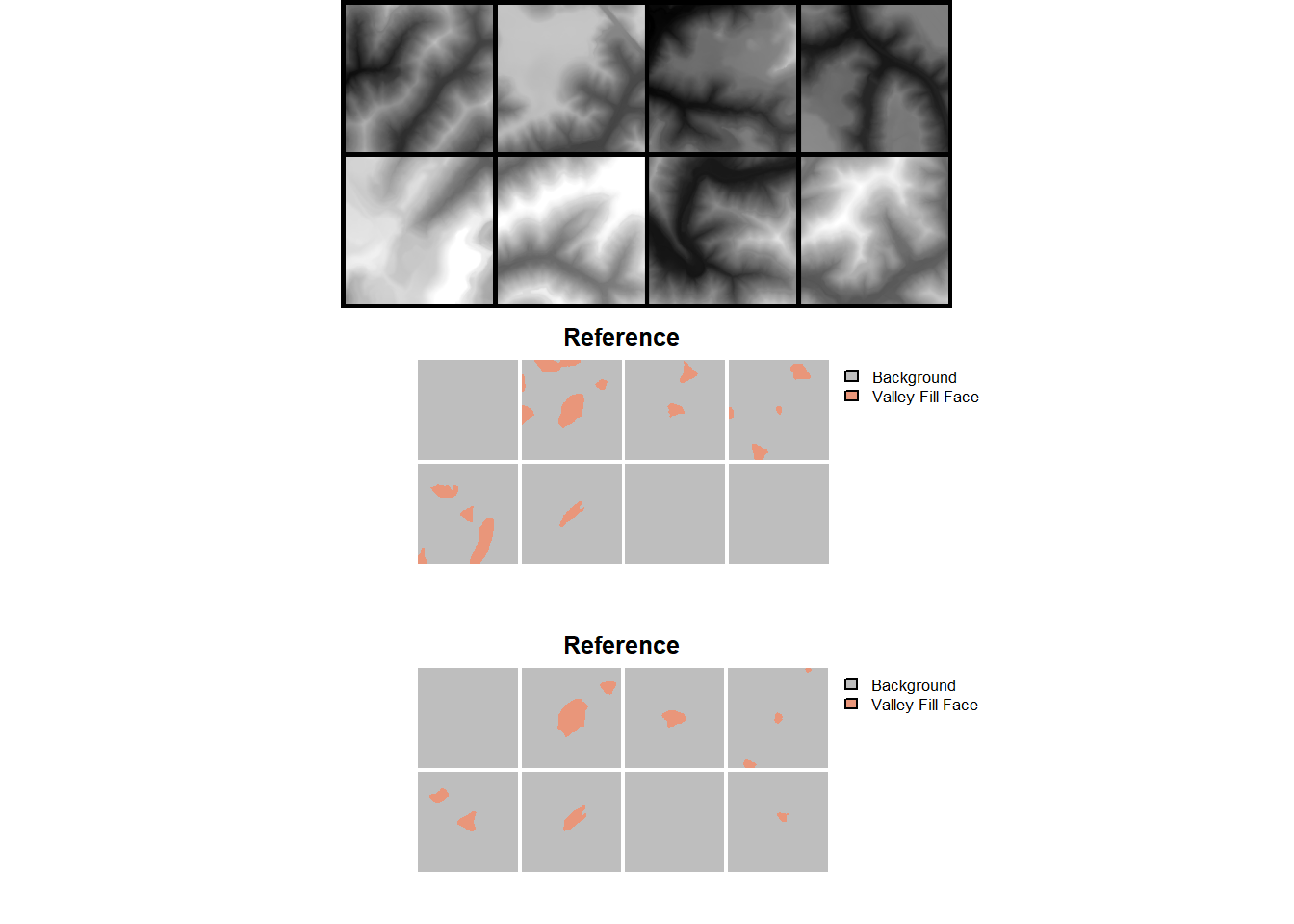
metricsOut <- assessDL(dl=testDL,
                       model=newModel,
                       batchSize=8,
                       size=640,
                       nCls=2,
                       multiclass=FALSE,
                       cropFactorMsk=64,
                       cropFactorPred=0,
                       cCodes=c(1,2),
                       cNames=c("Background", "Valley Fill Face"),
                       usedDS=FALSE,
                       useCUDA=TRUE,
                       decimals=4)

print(metricsOut)
$Classes
[1] "Background" "Valley Fill Face"
$referenceCounts
Negative Positive
263674365 15246851
$predictionCounts
Negative Positive
265854795 13066421
$ConfusionMatrix
Reference
Predicted Negative Positive
Negative 260796143 5058652
Positive 2878222 10188199
$Mets
OA Recall Precision Specificity NPV F1Score
Valley Fill Face 0.9715 0.6682 0.7797 0.9891 0.981 0.719716.4.5 Spatial Prediction
The predictSpatial() function is used to predict to a new spatial extent. The key difference here in comparison to Workflow 1 is that doPad should be set to TRUE and the prePad argument should match the tCrop argument used in defineTerrainSeg(). This will allow the predictions to align correctly when chips are merged into a final product. Note also that the input is now the DTM as opposed to the stack of LSPs since the model generates the LSPs internally. This is one of the key benefits of this workflow: LSPs, raster masks, and image chips do not need to be generated prior to training the model. The user simply needs to provide the input DTM, example vector features, and processing extents. Although generating chips and LSPs during training slows the process, pre-processing requirements are reduced, and the user does not need to generate LSPs prior to making a prediction to a new location.
predCls <-geodl::predictSpatial(imgIn="gslrData/chpt16/data/dtm.tif",
model=newModel,
predOut="gslrData/chpt16/data/vfillPredDynamic.tif",
mode="multiclass",
predType="class",
doPad = TRUE,
predPad = 64,
useCUDA= TRUE,
nCls=2,
chpSize=640,
stride_x=128,
stride_y=128,
crop=128,
nChn=1,
normalize=FALSE,
rescaleFactor=1,
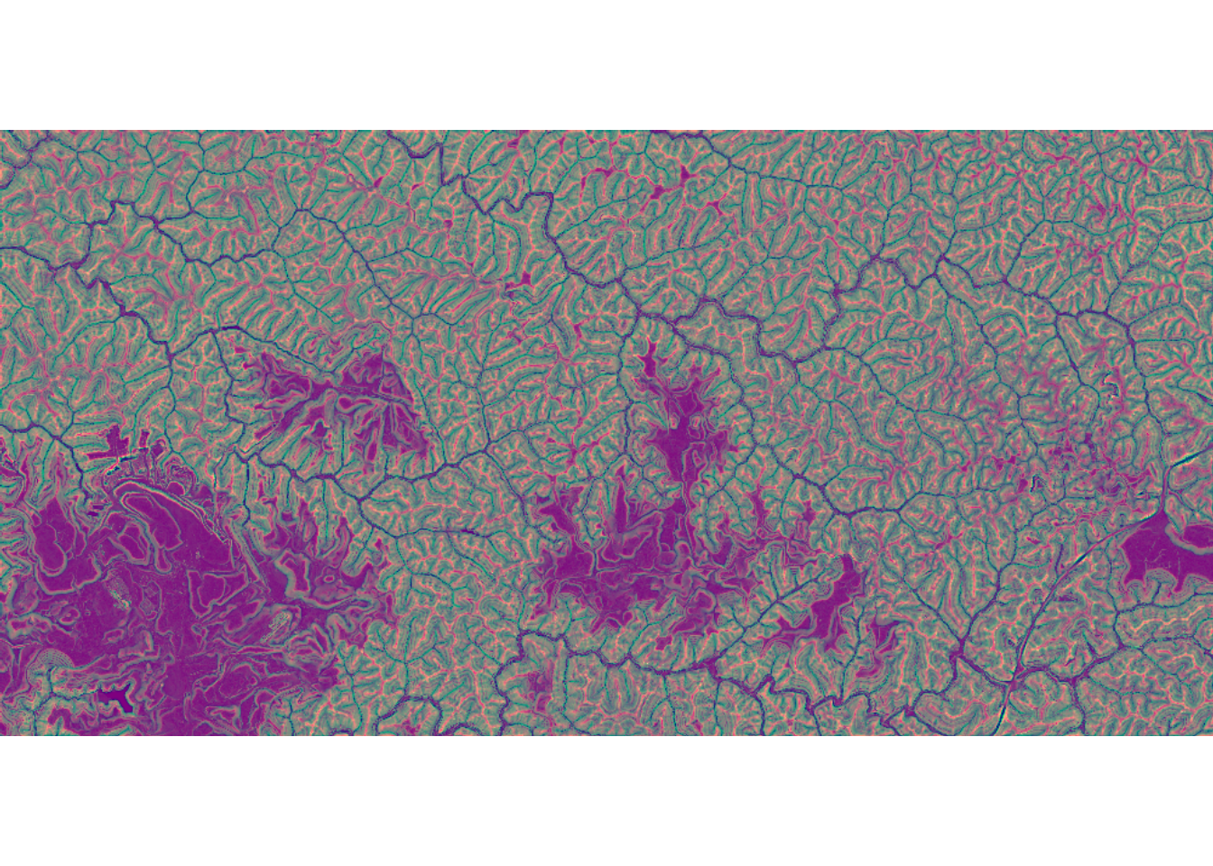
usedDS=FALSE)Lastly, we can visualize the predictions. We first generate a hillshade form the DTM then visualize the predictions over this surface. We convert codes of 0 and 1 to NA so that only the positive case cells are displayed.
dtm <- rast("gslrData/chpt16/data/dtm.tif")
slp <- terrain(dtm, v ="slope", unit="radians")
asp <- terrain(dtm, v ="aspect", unit="radians")

hs <- shade(slp, asp, angle=45, direction=315)

tm_shape(hs)+
  tm_raster(col.scale = tm_scale_continuous(values="-brewer.greys"))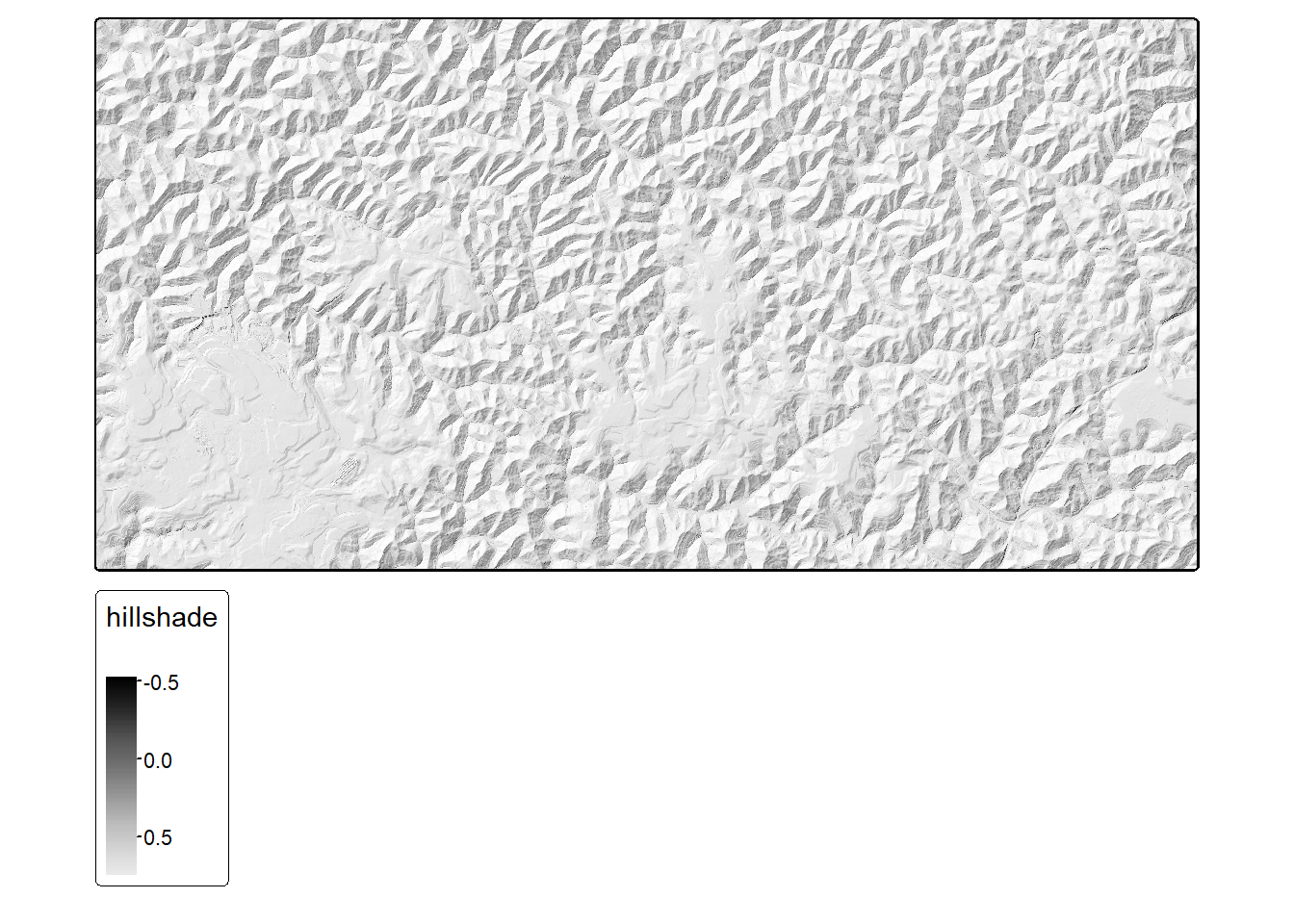
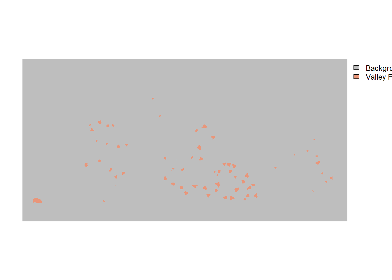
predCls <- rast("gslrData/chpt16/data/vfillPredDynamic.tif")

predCls2 <- predCls
predCls2[predCls2 == 0] <- NA
predCls2[predCls2 == 1] <- NA

tm_shape(hs)+
  tm_raster(col.scale = tm_scale_continuous(values="-brewer.greys"))+
  tm_shape(predCls2)+
  tm_raster(col.scale = tm_scale_categorical(labels = c("Valley Fill"),
                                             values = c("brown1")),
            col.legend = tm_legend("Features"))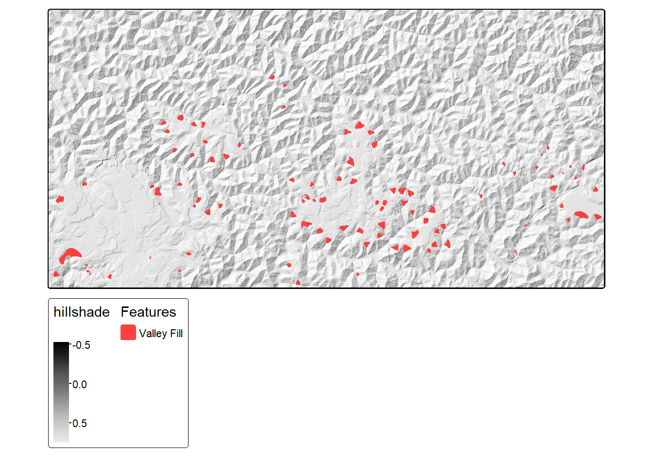
16.5 Workflow 3: Landcover.ai (Multiclass)
For this last example, we return to using pre-generated chips. However, we now explore a multiclass classification problem.
16.5.1 Preparation
We begin by reading in the required libraries and the data partition files provided by the data originators. Since these files were generated outside of the geodl workflow, we need to augment them. This simply requires generating “chpN”, “chpPth”, and “mskPth” columns that house the file name, relative path to the image chips, and relative path to the raster masks, respectively. To speed up our experiment, we also extract out a random subset of 3,000 training chips and 500 chips each from the validation and test sets. Finally, we visualize some random chips using viewChips() as a check.
If training a model for later use, we recommend using all of the training chips. We are simply subsetting the data here to speed up the example.
trainDF <- data.frame(chpN=trainDF$V1,
                      chpPth=paste0("images/", trainDF$V1, ".tif"),
                      mskPth=paste0("masks/", trainDF$V1, "_m.tif")) |>
  sample_frac(1, replace=FALSE) |> sample_n(3000)

testDF <- data.frame(chpN=testDF$V1,
                     chpPth=paste0("images/", testDF$V1, ".tif"),
                     mskPth=paste0("masks/", testDF$V1, "_m.tif")) |>
  sample_frac(1, replace=FALSE) |> sample_n(500)

valDF <- data.frame(chpN=valDF$V1,
                    chpPth=paste0("images/", valDF$V1, ".tif"),
                    mskPth=paste0("masks/", valDF$V1, "_m.tif"))  |>
sample_frac(1, replace=FALSE) |> sample_n(500)viewChips(chpDF=trainDF,
folder="E:/myFiles/data/landcoverai/train/",
nSamps = 25,
mode = "both",
justPositive = FALSE,
cCnt = 5,
rCnt = 5,
r = 1,
g = 2,
b = 3,
rescale = FALSE,
rescaleVal = 1,
cCodes= c(0,1,2,3,4),
cNames= c("Background",
"Buildings",
"Woodland",
"Water",
"Road"),
cColors= c("gray", "red", "green", "blue", "black"),
useSeed = TRUE,
seed = 42)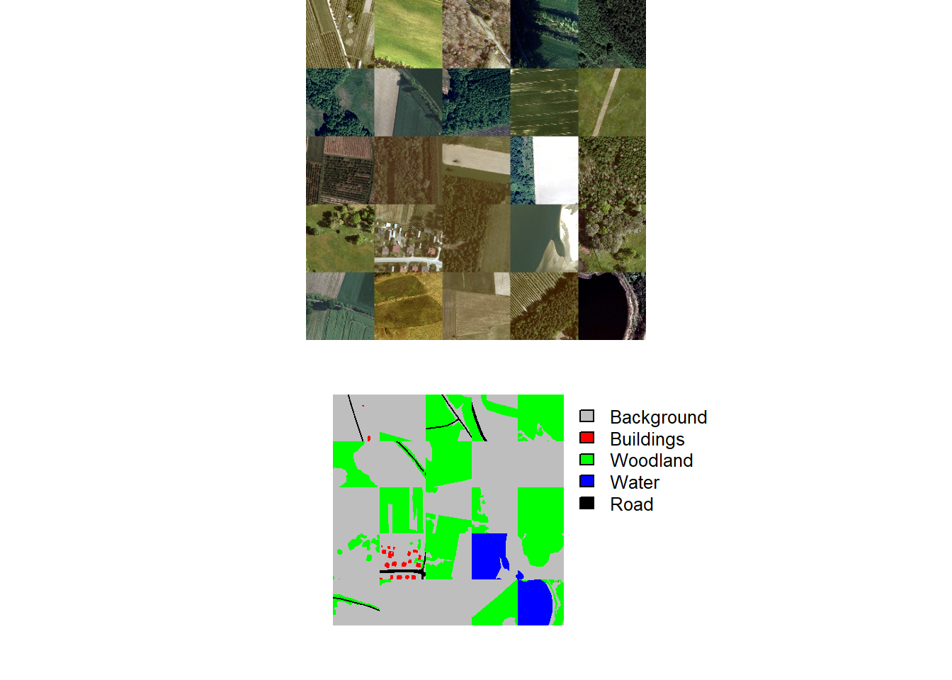
16.5.2 Datasets and Dataloaders
We next instantiate torch datasets for all three partitions. Since the input RGB imagery are unsigned 8-bit and scaled between 0 and 255, they are re-scaled from 0 to 1 using rescaleFactor=255. We also add 1 to the masks so that class codes are 1 to 5 as opposed to 0 to 4. Random vertical flips, horizontal flips, and rotations and random changes to brightness and saturation are applied to the training set. No augmentations are applied to the validation or test set.
trainDS <- defineSegDataSet(
  chpDF=trainDF,
  folder="E:/myFiles/data/landcoverai/train/",
  normalize = FALSE,
  rescaleFactor = 255,
  mskRescale= 1,
  bands = c(1,2,3),
  mskAdd=1,
  doAugs = TRUE,
  maxAugs = 1,
  probVFlip = .5,
  probHFlip = .5,
  probRotation=.3,
  probBrightness = .1,
  probContrast = 0,
  probGamma = 0,
  probHue = 0,
  probSaturation = .2,
  brightFactor = c(.9,1.1),
  contrastFactor = c(.9,1.1),
  gammaFactor = c(.9, 1.1, 1),
  hueFactor = c(-.1, .1),
  saturationFactor = c(.9, 1.1))

valDS <- defineSegDataSet(
  chpDF=valDF,
  folder="E:/myFiles/data/landcoverai/val/",
  normalize = FALSE,
  rescaleFactor = 255,
  mskRescale = 1,
  mskAdd=1)

testDS <- defineSegDataSet(
  chpDF=testDF,
  folder="E:/myFiles/data/landcoverai/test/",
  normalize = FALSE,
  rescaleFactor = 255,
  mskRescale = 1,
  mskAdd=1)
We next define torch dataloaders using a mini-batch size of 12. The last mini-batch is dropped, and only the training set is shuffled. Again, you may need to change the mini-batch size to run the example on your machine.
trainDL <- torch::dataloader(trainDS,
                             batch_size=12,
                             shuffle=TRUE,
                             drop_last = TRUE)

valDL <- torch::dataloader(valDS,
                           batch_size=12,
                           shuffle=FALSE,
                           drop_last = TRUE)

testDL <- torch::dataloader(testDS,
                            batch_size=12,
                            shuffle=FALSE,
                            drop_last = TRUE)
Lastly, we perform checks by plotting a mini-batch of the data using viewBatch() and obtain information about a mini-batch using describeBatch(). Since no issues are observed, we are now ready to train the model.
viewBatch(dataLoader=trainDL,
          nCols = 4,
          padding=30,
          r = 1,
          g = 2,
          b = 3,
          cCodes= c(1,2,3,4,5),
          cNames=c("Background",
                   "Buildings",
                   "Woodland",
                   "Water",
                   "Road"),
          cColors=c("gray", "red", "green", "blue", "black"))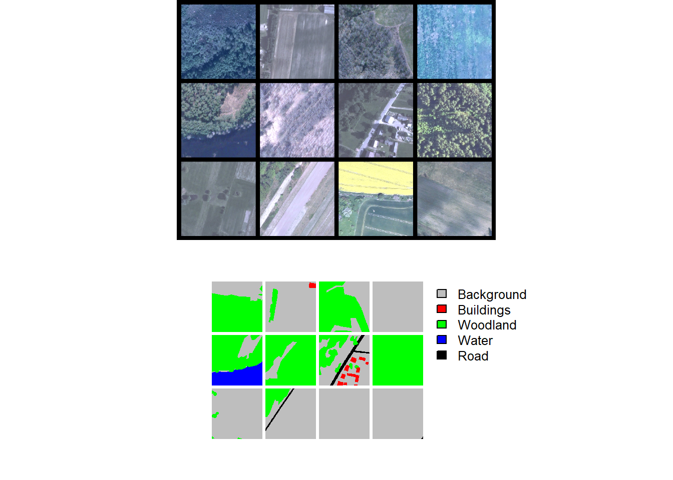
viewBatch(dataLoader=valDL,
          nCols = 4,
          padding=30,
          r = 1,
          g = 2,
          b = 3,
          cCodes = c(1,2,3,4,5),
          cNames=c("Background", "Buildings", "Woodland", "Water", "Road"),
          cColors=c("gray", "red", "green", "blue", "black"))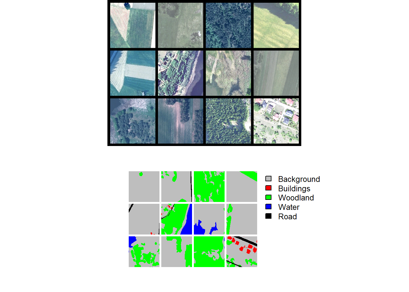
trainStats <- describeBatch(trainDL,
                            zeroStart=FALSE)
valStats <- describeBatch(valDL,
zeroStart=FALSE)print(trainStats)$batchSize
[1] 12
$imageDataType
[1] "Float"
$maskDataType
[1] "Long"
$imageShape
[1] "12" "3" "512" "512"
$maskShape
[1] "12" "1" "512" "512"
$bndMns
[1] 0.3732770 0.3901036 0.3325955
$bandSDs
[1] 0.1711579 0.1482689 0.1051226
$maskCount
[1] 1930338 66293 1086929 531 61637
$minIndex
[1] 1
$maxIndex
[1] 5print(valStats)$batchSize
[1] 12
$imageDataType
[1] "Float"
$maskDataType
[1] "Long"
$imageShape
[1] "12" "3" "512" "512"
$maskShape
[1] "12" "1" "512" "512"
$bndMns
[1] 0.3350235 0.3628660 0.3255590
$bandSDs
[1] 0.14951262 0.12114301 0.08688904
$maskCount
[1] 2121350 29318 852280 108354 34426
$minIndex
[1] 1
$maxIndex
[1] 516.5.3 Training Loop
We use a UNet architecture with a MobileNetv2 encoder as implemented with the defineMobileUNet() function. The architecture will differentiate 5 classes and expects 3 input predictor variables. We load pre-trained ImageNet parameters for the encoder but allow it to be updated during the training process (freezeEncoder = FALSE). We also use the leaky ReLU activation function throughout the architecture and define the desired number of output feature maps for each decoder block.
The loss is configured as a focal Dice loss (lambda = 0, gamma = 0.7, and delta = 0.5). All classes are equally weighted in the loss calculation. We also exclude outer rows and columns of cells for each chip when calculating the loss. Overall accuracy, F1-score, recall, and precision are calculated in multiclass mode using macro-averaging where each class has equal weight in the aggregated metric. As with the loss function, we do not consider outer rows and columns of cells in the assessment metric calculations.
We use the AdamW optimizer, train the model for 25 epochs, log losses and metrics to disk, and save the model state dictionary after each training epoch. luz implements GPU-based acceleration.
If you choose to run the training loop, it will take several hours to execute. We have provided a trained model in the data folder for the chapter if you would like to execute the post-training code without training a new model. The file is named “landcoveraiModel.pt.” We have also included the training logs: “landcoveraiTrainingLogs.csv”. If you want to load our saved state dictionary, your model must use the exact same configuration as we have specified below.
device <- "cuda"

fitted <- defineMobileUNet |>
  luz::setup(
    loss = defineUnifiedFocalLoss(nCls=5,
                                  cropFactorPred=32,
                                  cropFactorMsk = 32,
                                  lambda=0,
                                  gamma=.7,
                                  delta=0.5,
                                  smooth = 1e-8,
                                  zeroStart=FALSE,
                                  clsWghtsDist=1,
                                  clsWghtsReg=1,
                                  useLogCosH =FALSE,
                                  device="cuda"),
    optimizer = optim_adamw,
    metrics = list(
      luz_metric_overall_accuracy(nCls=5,
                                  cropFactorPred=32,
                                  cropFactorMsk=32,
                                  smooth=1,
                                  mode = "multiclass",
                                  zeroStart= FALSE),
      luz_metric_f1score(nCls=5,
                         cropFactorPred=32,
                         cropFactorMsk=32,
                         smooth=1,
                         mode = "multiclass",
                         zeroStart= FALSE),
      luz_metric_recall(nCls=5,
                        cropFactorPred=32,
                        cropFactorMsk=32,
                        smooth=1,
                        mode = "multiclass",
                        zeroStart= FALSE),
      luz_metric_precision(nCls=5,
                           cropFactorPred=32,
                           cropFactorMsk=32,
                           smooth=1,
                           mode = "multiclass",
                           zeroStart= FALSE)
    )
  ) |>
  set_hparams(inChn=3,
              nCls = 5,
              pretrainedEncoder = TRUE,
              freezeEncoder = FALSE,
              avgImNetWeights = FALSE,
              actFunc = "lrelu",
              useAttn = FALSE,
              useDS = FALSE,
              dcChn = c(256,128,64,32,16),
              negative_slope = 0.01) |>
  set_opt_hparams(lr = 1e-3,
  ) |>
  fit(data = trainDL,
      epochs = 25,
      valid_data = valDL,
      callbacks = list(luz_callback_csv_logger("D:/landcoverai/modelsV2/trainLogs.csv"),
                       callback_save_model_state_dict("D:/landcoverai/modelsV2/",
                                                      prefix = "epoch")),
      accelerator = accelerator(device_placement = TRUE,
                                cpu = FALSE,
                                cuda_index = torch::cuda_current_device()),
      verbose=TRUE)
16.5.4 Model Validation
As with the prior two workflows, we first visualize the losses and metrics over the training epochs. Some instability is noted towards the end of the model. We use the model state after epoch 7 as the final model.
allMets <- read.csv("gslrData/chpt16/data/landcoveraiTrainingLogs.csv")

ggplot(allMets, aes(x=epoch, y=loss, color=set))+
  geom_line(lwd=1)+
  labs(x="Epoch", y="Loss", color="Set")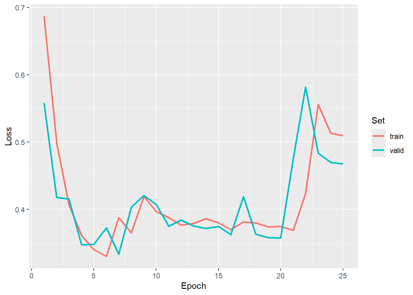
ggplot(allMets, aes(x=epoch, y=f1score, color=set))+
  geom_line(lwd=1)+
  labs(x="Epoch", y="F1-Score", color="Set")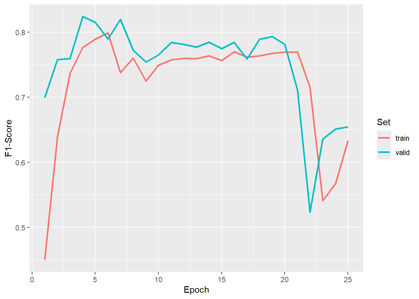
ggplot(allMets, aes(x=epoch, y=recall, color=set))+
  geom_line(lwd=1)+
  labs(x="Epoch", y="Recall", color="Set")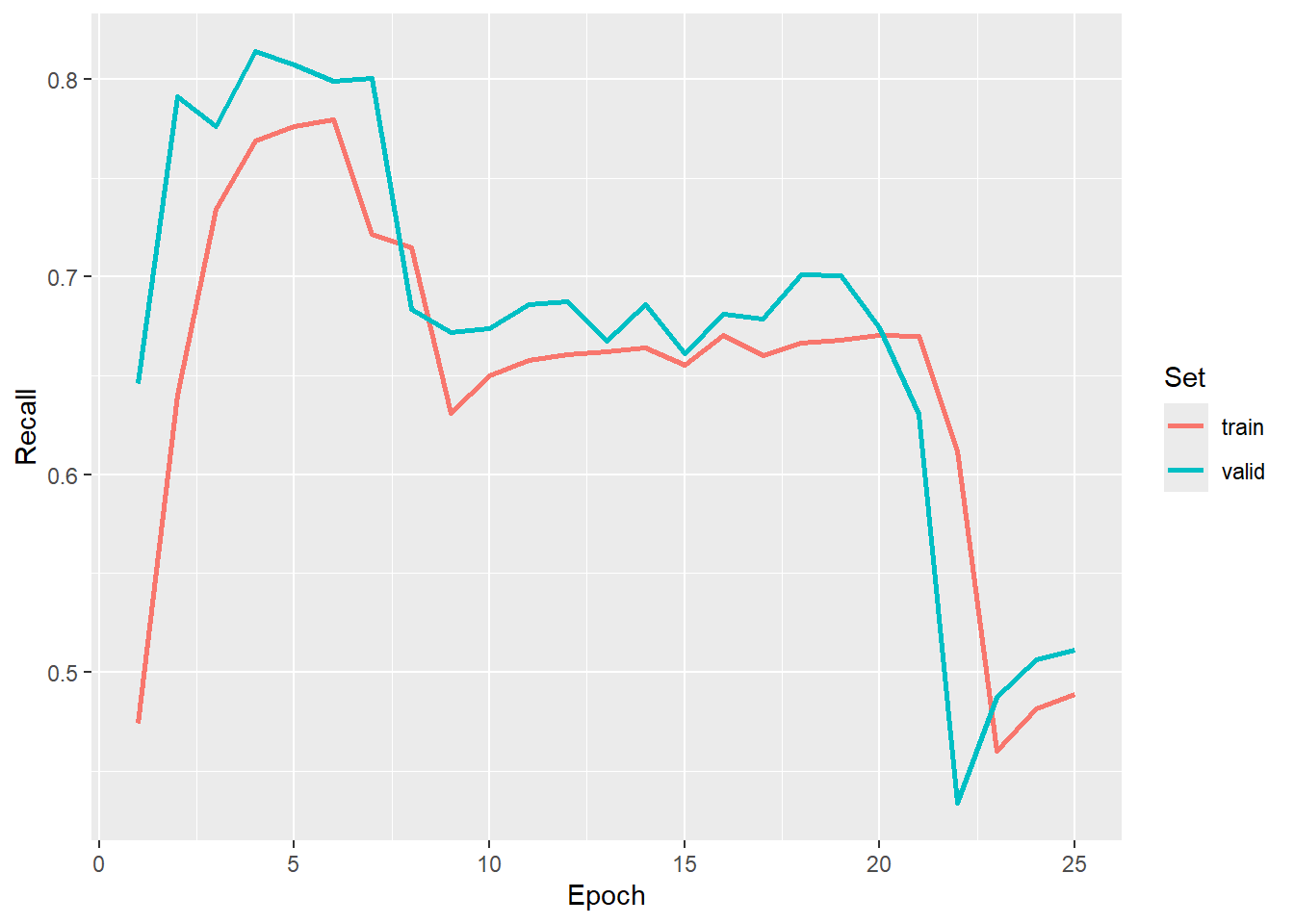
ggplot(allMets, aes(x=epoch, y=precision, color=set))+
  geom_line(lwd=1)+
  labs(x="Epoch", y="Precision", color="Set")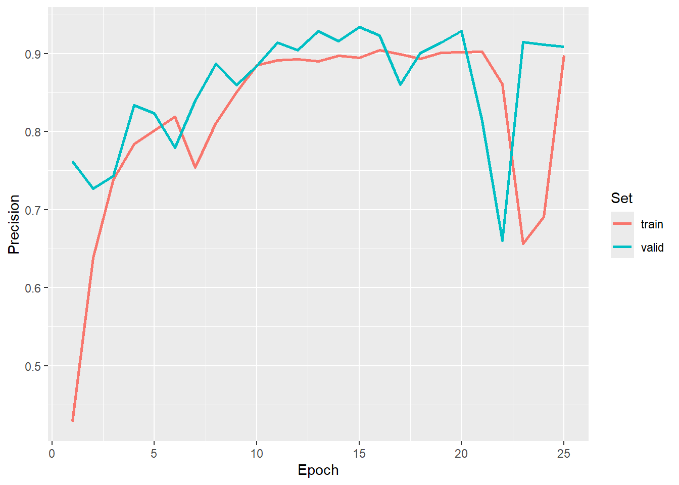
We re-instantiate the model, load the saved state dictionary, and place it in evaluation mode. Again, the new model must have the exact same configuration as the model that was trained above in order for the state dictionary to be loaded correctly.
newModel <-   defineMobileUNet(inChn=3,
                               nCls = 5,
                               pretrainedEncoder = TRUE,
                               freezeEncoder = FALSE,
                               avgImNetWeights = FALSE,
                               actFunc = "lrelu",
                               useAttn = FALSE,
                               useDS = FALSE,
                               dcChn = c(256,128,64,32,16),
                               negative_slope = 0.01)

newModel$load_state_dict(torch_load(str_glue("gslrData/chpt16/data/landcoveraiModel.pt")))$to(device="cuda")
newModel$eval()
Once the model is prepared, we visualize a mini-batch of predictions using viewBatchPreds(). We then obtain assessment metrics for all mini-batches using assessDL().
viewBatchPreds(dataLoader=testDL,
               model=newModel,
               mode="multiclass",
               padding=30,
               nCols = 4,
               r = 1,
               g = 2,
               b = 3,
               cCodes=c(1,2,3,4,5),
               cNames=c("Background", "Buildings", "Woodland", "Water", "Road"),
               cColors=c("gray", "red", "green", "blue", "black"),
               useCUDA=TRUE,
               probs=FALSE,
               usedDS=FALSE)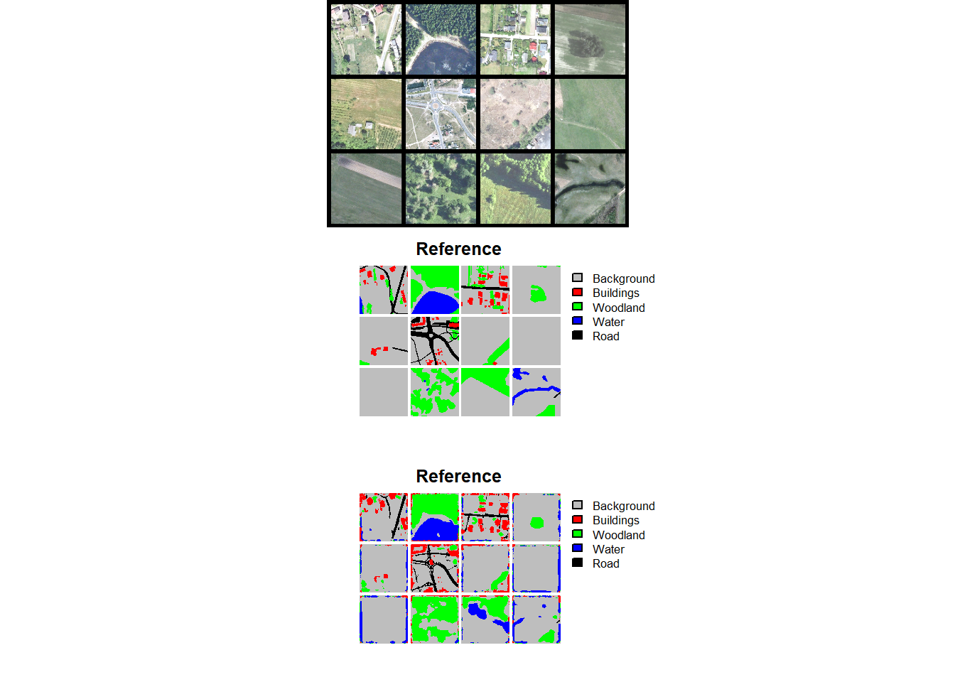
testEval2 <- assessDL(dl=testDL,
                      model=newModel,
                      batchSize=12,
                      size=512,
                      nCls=5,
                      multiclass=TRUE,
                      cCodes=c(1,2,3,4,5),
                      cNames=c("Background", "Buildings", "Woodland", "water", "road"),
                      usedDS=FALSE,
                      useCUDA=TRUE)

print(testEval2)
$Classes
[1] "Background" "Buildings" "Woodland" "water" "road"
$referenceCounts
Background Buildings Woodland water road
74359505 1329119 2463060 7063564 43759600
$predictionCounts
Background Buildings Woodland water road
70906883 5113203 1510370 10736997 40707395
$confusionMatrix
Reference
Predicted Background Buildings Woodland water road
Background 62598613 239819 901390 848265 6318796
Buildings 2339571 1003265 171793 183341 1415233
Woodland 301187 27654 1177966 1284 2279
water 4756183 3617 6038 5772530 198629
road 4363951 54764 205873 258144 35824663
$aggMetrics
OA macroF1 macroPA macroUA
1 0.8248 0.696 0.7422 0.6553
$userAccuracies
Background Buildings Woodland water road
0.8828 0.1962 0.7799 0.5376 0.8801
$producerAccuracies
Background Buildings Woodland water road
0.8418 0.7548 0.4783 0.8172 0.8187
$f1Scores
Background Buildings Woodland water road
0.8618 0.3115 0.5929 0.6486 0.8483 16.5.5 Spatial Predictions
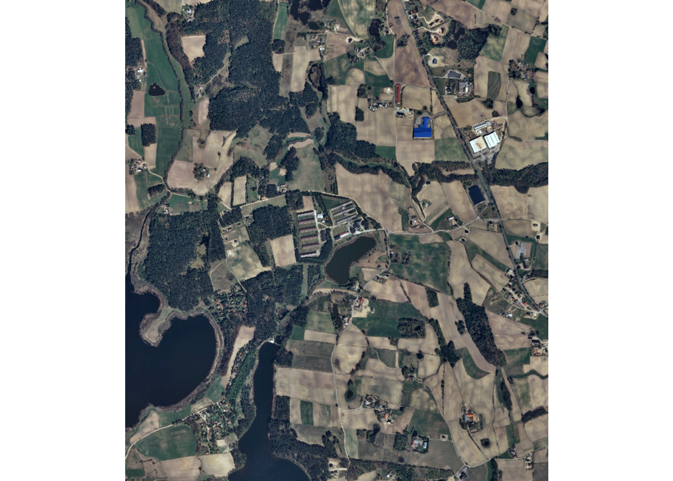
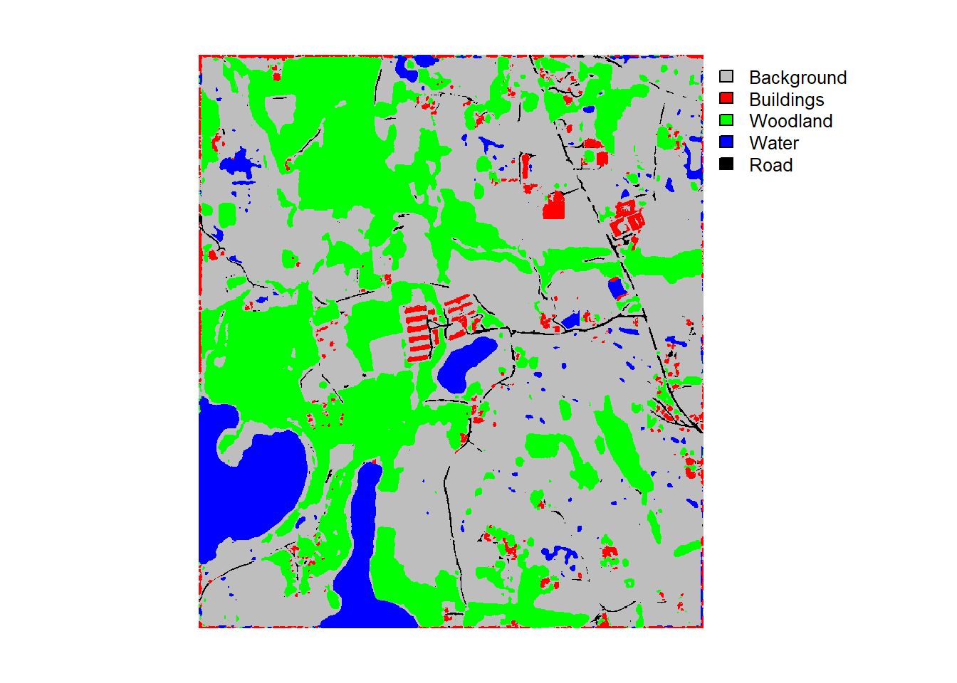
The final model can be used to predict to new data using the predictSpatial() function. The test image (“landcoveraiIMG.tif”) has been provided in the data folder for the chapter along with an example prediction (“landcoveraiPred.tif”). Note that the image is re-scaled using rescaleFactor=255. It is important that the new data are processed using the same configuration as the data used to train the model and generated using the dataset subclass.
predCls <- predictSpatial(imgIn="gslrData/chpt16/data/landcoveraiIMG.tif",
                          model=newModel,
                          predOut="gslrData/chpt16/data/landcoveraiPred.tif",
                          mode="multiclass",
                          predType="class",
                          useCUDA=TRUE,
                          nCls=5,
                          chpSize=512,
                          stride_x=256,
                          stride_y=256,
                          crop=50,
                          nChn=3,
                          normalize=FALSE,
                          rescaleFactor=255,
                          usedDS=FALSE)
Lastly, we visualize the input image and its associated prediction.
16.6 Concluding Remarks
We hope that the three example workflows provided here will aid you in using the goedl package for your own geospatial semantic segmentation tasks. One benefit of this package is that it simplifies the use of torch for performing geospatial semantic segmentation. The process is implemented using functions and a declarative structure as opposed to generating custom subclasses of torch classes. This package is still in active development, so please remember to check for updates.
16.7 Questions
- Why should you monitor a validation set during the training process?
- Why is it common to implement data augmentations for the training set?
- Explain the purpose of the
drop_lastparameter in the torch dataloader. Why might you need to drop the last mini-batch? - Explain why it is generally best to start class indices at 1 as opposed to 0 for multiclass classification using torch in R.
- Why is it necessary that a new instantiation of a model have the same architecture if we want to be able to load a state dictionary that was saved to disk?
- Explain the difference between a “hard” and “soft” prediction.
- geodl generally frames all problems as multiclass. How can the F1-score, recall, and precision assessment metrics be configured to provide a binary-style estimate as opposed to a macro-average of the background and presence classes?
- Why might we want to exclude margin rows and columns when calculating a loss or assessment metrics?
16.8 Exercises
Develop a pipeline to train and evaluate a geospatial semantic segmentation model using geodl, torch and luz. The goal of the model is to extract the extent of historic surface mines from topographic maps. You will make use of the topoDLMini dataset, which is available here. These data were introduced in the following publication, which is available here and is in open access:
Maxwell, A.E., Bester, M.S., Guillen, L.A., Ramezan, C.A., Carpinello, D.J., Fan, Y., Hartley, F.M., Maynard, S.M. and Pyron, J.L., 2020. Semantic segmentation deep learning for extracting surface mine extents from historic topographic maps. Remote Sensing, 12(24), p.4145.
Generate code to perform the following steps. Note that a CUDA-enabled GPU is required to complete this exercise.
- Use
makeChipsDF()to generate the chips data frames. The topoDLMini folder contains separate train, val, and test folders and were generated withmakeChips()in “Divided” mode. The file extension is “.png”. The generated training, validation, and test data frames should list 2,000, 500, and 500 chips, respectively. - Instantiate torch datasets for each partition using
defineSegDataSet(). Note that the image chips need to be re-scaled from 0 to 255 to 0 to 1. The masks also need to be re-scaled from 0 to 255 to 0 to 1. You should also add 1 to the class codes to obtain codes of 1 and 2 (1 = “background”; 2 = “mine”). For the training set, perform some augmentations of your choosing to help combat overfitting. - Generate torch dataloaders with a mini-batch size of 10 for all data partitions (note that you may need to lower the mini-batch size depending on your available hardware). Shuffle the training set. If using a mini-batch size of 10, you do not need to drop the last mini-batch. However, if you use an alternative mini-batch size and the number of chips is not evenly divisible by the mini-batch size, you should drop the last mini-batch.
- Check the data using
viewBatch()anddescribeBatch(). Note that the images should be scaled from 0 to 1, the the mask codes should be 1 and 2, there should be 3 input channels, and the spatial dimensions should be 256x256. If this is not the case, check your parameterization ofdefineSegDataSet(). - Train a model using luz. Use the training dataloader to train the model and the validation dataloader for validation. Use a UNet3+ model via
defineUNet3p()that is parameterized to predict 2 classes and accept 3 predictor variables. You can use the default arguments for all other parameters. Use the adamw optimizer with a learning rate of 0.001. Use a focal Tversky loss via thedefineUnifiedFocalLoss()function withlambda=0,gamma=0.7, anddelta=0.6. Use class weights ofc(0.3, 0.7). Monitor overall accuracy, F1-score, recall, and precision. Make sure to parameterize F1-score, recall, and precision as expected for a binary classification usingclsWghts=c(0,1). Train the model for 25 epochs, log the loss and metrics to disk, and save the model state dictionary at the end of each epoch. - Use the logs to select a final model.
- Re-instantiate the model with the same configuration and load the saved state dictionary representing the epoch that you selected. Make sure to place the model in evaluation mode.
- Validate the model on the test set using
assessDL(). - View a mini-batch of predictions for the test set using
viewBatchPreds() - Generate a short write up of your results. Discuss issues of commission and omission errors.