8 Introduction to Machine Learning (tidymodels)
8.1 Topics Covered
- Purpose of different packages included in the tidymodels metapackage
- Understand the tidymodels basic workflow
- Define and fit a model using parsnips
- Create data partitions using rsample
- Prepare data using recipes
- Assess models using yardstick
- Apply a trained model to raster data and post-process the result
8.1.1 Intro to tidymodels
The goal of this and the following chapter is to explore the tidymodels framework or metapackage for developing machine learning (ML) workflows in R. Different ML algorithms are implemented within different R packages; for example, random forest (RF) is implemented by both the randomForest and ranger packages. Unfortunately, different packages tend to use different workflows and syntax, making it difficult to experiment with or compare different ML algorithms, preprocessing routines, feature spaces, and/or hyperparameter combinations. The goal of tidymodels is to make it easier to implement ML in R and compare different algorithms and/or pipelines using a common philosophy and syntax. tidymodels is a metapackage constituted by a set of packages that compartmentalize different components of the ML workflow. The primary packages are:
- parsnips: implements a variety of ML algorithms using consistent syntax by calling to other R packages
- recipes: preprocessing and feature engineering
- rsample: data splitting and resampling
- tune: model optimization and hyperparameter tuning
- dials: define and manage hyperparameter settings to test
- workflows: define and implement a unified workflow consisting of preprocessing, tuning, training, and post-processing components
- yardstick: accuracy assessment and model validation
- broom: model management
Other than the core set of packages, tidymodels is expanded by additional packages including:
- infer: statistical inference using tidymodels syntax
- corrr: work with correlation matrices
- worflowsets: combine multiple workflows
- baguette: use bagging to create model ensembles
- stacks: generate stacked ensemble models
- finetune: additional hyperparameter tuning functionality to expand upon the functionality provided by the tune package
- spatialsample: spatial methods for resampling and data partitioning
- probably: post-process probability estimates
- tidyposterior: statistically compare models using Bayesian and resampling methods
- discrim: discriminant analysis models
- plsmod: linear projection models
- rules: rule-based models
- multilevelmod: multi-level or hierarchical models
- embed: generate embeddings or projections for predictor variables
- textrecipes: text preprocessing
- tidypredict: convert a model to a different programming language or for use in a database
- shinymodels: use Shiny, or an interactive web app, to explore model tuning or resampling results
- butcher: reduce the size of a model when saved to disk
- hardhat: assist developers in contributing to the tidymodels ecosystem
In this chapter, we explore two basic workflows:
- Workflow 1: define and train a model and make predictions
- Workflow 2: implement preprocessing and accuracy assessment
In the next chapter, we explore two more advanced workflows:
- Workflow 3: use workflows to simplify the model development pipeline and implement hyperparameter tuning
- Workflow 4: train, tune, and compare multiple model/preprocessing combinations using a workflow set
8.1.2 About the Example Data
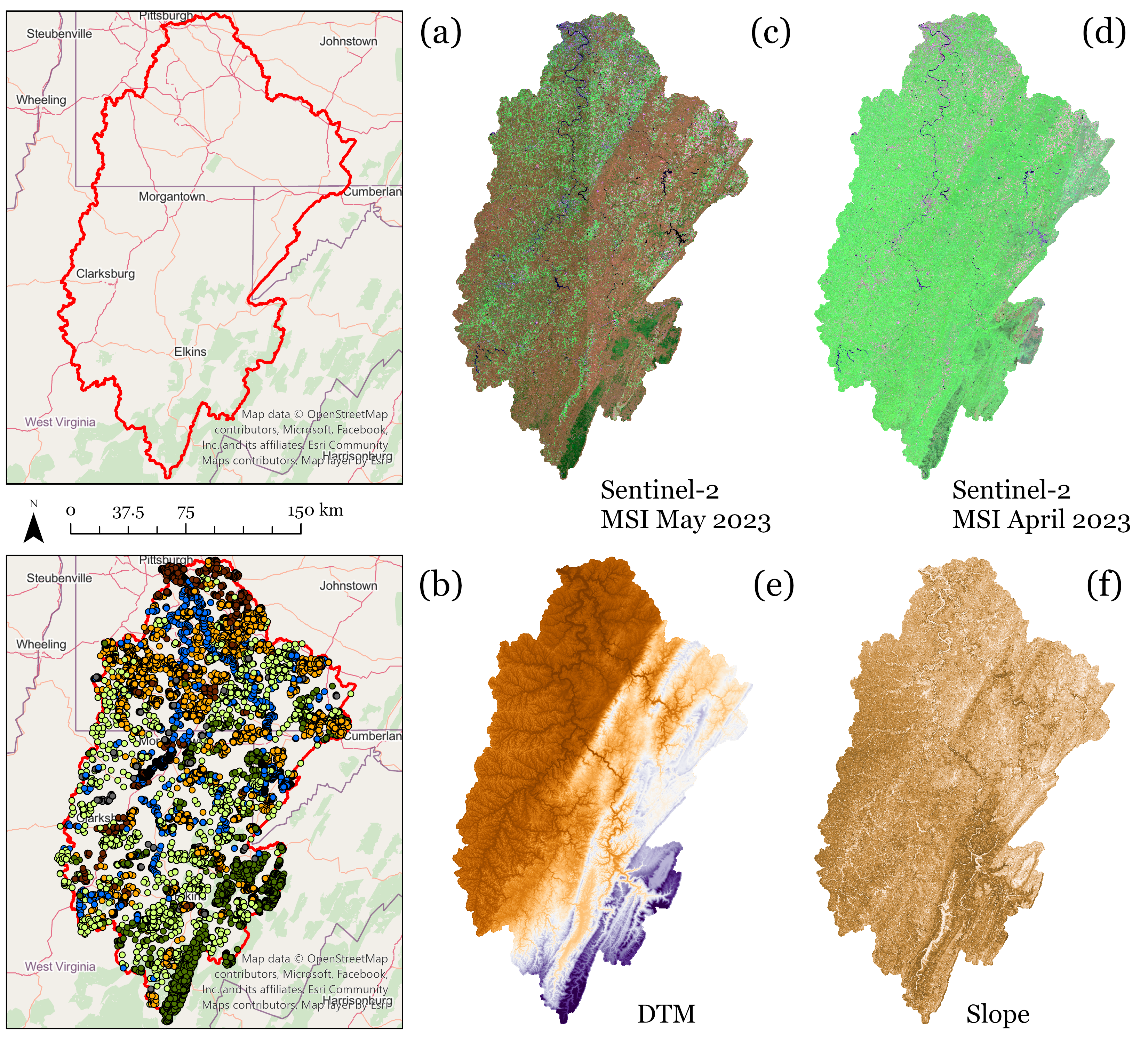
We will primarily make use of the Monongahela River Watershed land cover dataset. This watershed encompass portions of north central West Virginia, western Maryland, and southwestern Pennsylvania. This is a multiclass problem where the predictor variables consist of image band digital number (DN) values for data collected by the Sentinel-2 Multispectral Instrument (MSI) sensor in April 2023 (leaf-off conditions) and May 2023 (leaf-on conditions). We also include elevation, topographic slope, and a topographic position index (TPI) as additional predictor variables. Elevation data were provided by the United States Geological Survey (USGS) National Elevation Dataset (NED). These data were originally generated by students who participated in the Summer 2023 West Virginia Governor’s Computer Science Institute. Additional information about this project can be found here.
The figure below shows (a) the watershed boundary, (b) the labeled sample points collected by the students via heads-up data interpretation, (c) the April imagery, (d) the May imagery, (e) the NED elevation data, and (f) topographic slope. All data were processed at a 10 m spatial grain. For this study, we used MSI bands 2, 3, 4, 5, 6, 7, 8, 8A, 11, and 12 (i.e., blue, green, red, red edge 1, red edge 2, red edge 3, near infrared (NIR), NIR narrow, shortwave infrared 1 (SWIR1), and SWIR2). As a result, we used ten bands for both image dates plus three topographic variables for a total of 23 predictor variables. The following classes were differentiated: barren, conifer forest, deciduous forest, developed, grass, and water. A total of 12,023 samples were generated. Note that one issue with this dataset is that the samples were not collected using randomized, unbiased methods. As a result, the accuracy assessments we will perform are biased. However, the data are adequate to demonstrate the use of tidymodels.
8.1.3 Load Packages
The following packages/metapackages are required for this chapter:
- tidymodels
- tidyverse
- terra
- tmap
- tmaptools
- micer
- gt
The tidyverse packages are used for basic data wrangling and manipulation. terra is used for reading and handling raster-based geospatial data. tmap is used for generating map output while tmaptools provides additional functionality to accompany tmap. micer implements the map image classification efficacy (MICE) metric. gt is used for table generation.
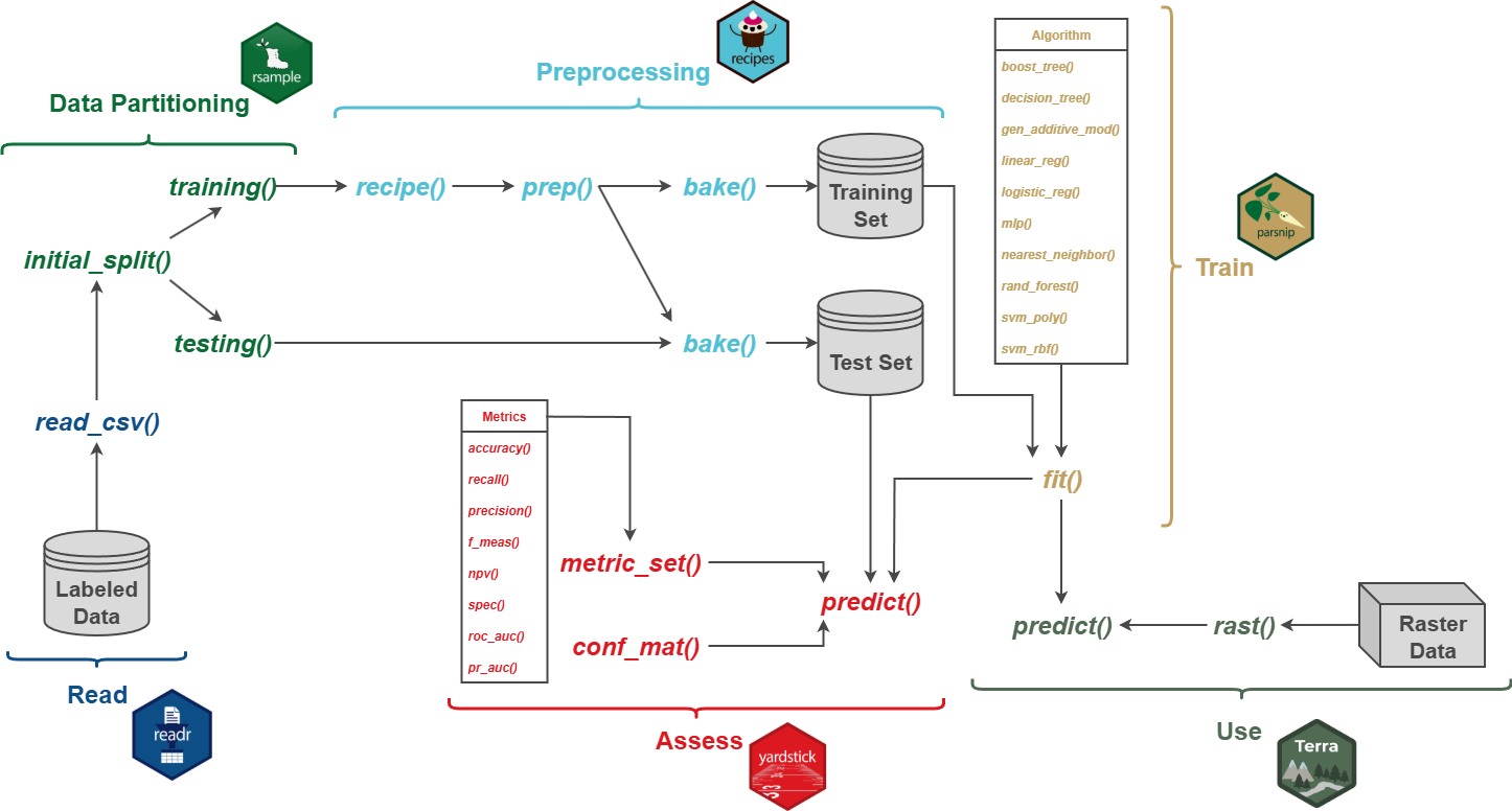
8.2 Workflow 1
We begin with a very simple workflow that only includes reading in labeled data as a table using readr, which is part of the tidyverse, defining and fitting a model with parsnips, and using the model to make predictions for all cells in a raster extent using terra. Figure 8.1 conceptualizes this process.
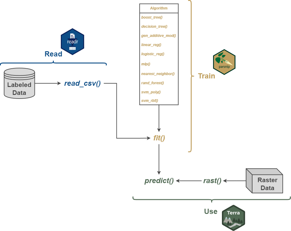
We first read in the data table using read_csv() from the readr package. The table includes the class names in the “lcClass” column along with all the predictor variables. The dplyr package, which is part of the tidyverse, is used to (1) convert all character columns to a factor data type, (2) remove unnecessary columns, and (3) drop any row or observation with missing data.
Before we proceed, let’s take some time to explore the data. Using the levels() function from base R, we can see that there are six different classes differentiated:
- “barren” = Barren
- “conForest” = Coniferous Forest
- “decForest” = Deciduous Forest
- “developed” = Developed
- “grass” = Pasture/Herbaceous/Low Vegetation
- “water” = Water
glimpse() provides a summary of the table. All columns ending in “_apr” represent the bands from the leaf-off, April image while those ending with “_may” are from the leaf-on, May image. All predictor variables are being treated as numeric data.
It is generally a good idea to explore your data prior to starting your analysis or modeling workflow.
levels(monD$lcClass)[1] "barren" "conForest" "decForest" "developed" "grass" "water" monD |>
glimpse()Rows: 12,032
Columns: 24
$ lcClass <fct> decForest, grass, grass, grass, grass, grass, grass, grass, co…
$ b1_apr <dbl> 1383.726, 1603.000, 1446.496, 1628.558, 1599.838, 1546.803, 14…
$ b2_apr <dbl> 1512.086, 1928.000, 1776.102, 1925.813, 1866.072, 1828.438, 17…
$ b3_apr <dbl> 1660.469, 1988.000, 1712.788, 2041.557, 1991.843, 1938.717, 17…
$ b4_apr <dbl> 2697.562, 4199.000, 4778.581, 4086.665, 3724.652, 4209.023, 45…
$ b5_apr <dbl> 2036.568, 2552.000, 2403.971, 2460.532, 2444.914, 2498.400, 24…
$ b6_apr <dbl> 2392.931, 3598.000, 3956.934, 3549.943, 3282.715, 3619.253, 38…
$ b7_apr <dbl> 2574.489, 3937.000, 4446.714, 3892.034, 3556.715, 3971.253, 42…
$ b8_apr <dbl> 2869.811, 4273.000, 4824.034, 4192.971, 3848.534, 4301.427, 46…
$ b9_apr <dbl> 3554.657, 4179.000, 3825.714, 3994.382, 4354.946, 4266.293, 38…
$ b10_apr <dbl> 2692.952, 2891.000, 2543.423, 2822.499, 3038.851, 2890.800, 26…
$ b1_may <dbl> 1255.533, 1350.000, 1340.982, 1332.018, 1398.115, 1334.782, 13…
$ b2_may <dbl> 1557.283, 1694.000, 1615.059, 1594.534, 1692.209, 1634.715, 16…
$ b3_may <dbl> 1203.855, 1392.000, 1358.233, 1370.480, 1497.099, 1386.995, 14…
$ b4_may <dbl> 5325.783, 5041.000, 5268.438, 4945.016, 4689.420, 5065.692, 51…
$ b5_may <dbl> 2112.773, 2234.000, 2114.461, 2006.573, 2188.862, 2164.459, 21…
$ b6_may <dbl> 4599.831, 4141.000, 4229.606, 4061.413, 3967.927, 4119.977, 42…
$ b7_may <dbl> 5531.103, 4726.000, 4927.063, 4749.184, 4464.084, 4751.642, 48…
$ b8_may <dbl> 5609.951, 5014.000, 5345.684, 5072.960, 4778.817, 5115.112, 51…
$ b9_may <dbl> 2891.510, 3080.000, 2997.397, 2828.392, 3341.547, 3215.812, 31…
$ b10_may <dbl> 1817.483, 2019.000, 1917.773, 1878.105, 2179.672, 2058.388, 20…
$ elev <dbl> 1090.1238, 993.7653, 981.2296, 983.3743, 984.1840, 1044.6538, …
$ slp <dbl> 20.884466, 11.969959, 4.584695, 11.660369, 3.733045, 7.216317,…
$ tpi <dbl> -3.3176472, 0.1519503, 0.0298904, -0.2036612, -0.1007883, 0.18…Counting the number of samples per class, we can see that there is notable class imbalance. As a result, we perform stratified random sampling without replacement to select an equal number of samples, 880, per class. This is accomplished using functions made available by dplyr.
# A tibble: 6 × 2
# Groups:   lcClass [6]
  lcClass       n
  <fct>     <int>
1 barren      885
2 conForest  2220
3 decForest  1639
4 developed  1061
5 grass      4226
6 water      2001
We use set.seed() throughout our code to make random processes deterministic for reproducibility.
8.2.1 Define and Train Models
We can now use parsnips to define models to train. We demonstrate how to configure three different algorithms: random forest (RF), a support vector machine (SVM), and k-nearest neighbors (kNN). We first define the models, which includes specifying hyperparameters and setting the engine and mode. It is necessary to set an engine if parsnips interfaces with multiple packages that implement the algorithm of interest. For example, RF is implemented with both randomForest and ranger, among other packages, and we have chosen to use the ranger implementation here. The mode is set to "classification" since we are predicting categories as opposed to a continuous variable. The hyperparameters that can be set vary between algorithms. Again, one of the benefits of parsnips is that it standardizes the names of hyperparameters across different implementations of the algorithm from different packages. Note also that there may be engine-specific settings that can be defined.
For the RF model, we use 500 trees in the ensemble and the default setting for all other hyperparameters, such as the number of random variables to select from at each decision node (mtry). For SVM, we use the kernlab package, a radial basis function (RBF) kernel, and the default values for the cost and rbf_sigma hyperparameters. For kNN, we use 11 neighbors. It is best practice to tune hyperparameters as opposed to using the default settings. We will demonstrate this in Workflows 3 and 4 in the next chapter. We are skipping this process here to simplify the workflow.
rfSpec <- rand_forest(trees=500) |>
  set_engine("ranger") |>
  set_mode("classification")

svmSpec <- svm_rbf() |>
  set_engine("kernlab") |>
  set_mode("classification")

knnSpec <- nearest_neighbor(neighbors=11) |>
  set_engine("kknn") |>
  set_mode("classification")
Once models are defined, they can be trained using the fit() function from parsnips, which results in a fitted model that can be used to make predictions to new data. Training the algorithm to create a model requires defining (1) the dependent variable and set of predictor variables and (2) the training dataset. The formula syntax (lcCLass ~ .) can be read as follows: “lcClass is predicted by all other variables in the table”. The column to the left of “~” is the variable being predicted, or the dependent variable, while variable(s) to the right of “~” are the predictor variables. When using all other columns in the table other than the dependent variable as predictor variables, “.” is used as a shorthand to indicate this so that you do not have to list out all the column names. If you need to use a subset of variables, you can either (1) remove unneeded variables from the table, as was demonstrated above, or (2) list out the variables as follows: Dependent Variable ~ Predictor 1 + Predictor 2 + Predictor 3.
rfModel <- rfSpec |>
  fit(lcClass ~.,
      data=trainDF)
8.2.2 Use Model
8.2.2.1 Predict to Raster Grid
Now that we have trained models, we will use them to make predictions to a raster dataset. We first read in a raster stack of the predictor variables for a subset of the entire watershed using the rast() function from terra and rename the bands to match the names used in the table.
If you plan to use a trained model to make predictions to a raster stack, it is important to rename the bands to match the names used in the table. Make sure you know which band represents each predictor variable. Also, we generally find it easier to stack all of the predictor variables into a single file using GIS software prior to reading them into R since R is very unforgiving in regards to different origins, cell sizes, and/or count of rows/columns of pixels. In other words, data need to align perfectly.
If we call the name of the generated spatRaster object, we can obtain information about the raster stack. The data consists of 3,669 rows and 3,224 columns of values with a total of 23 bands or layers, as expected. It has a cell size of ~ 10 m and is referenced to the WGS84 datum and the Web Mercator projection.
stkclass : SpatRaster
dimensions : 3669, 3224, 23 (nrow, ncol, nlyr)
resolution : 9.999732, 9.999871 (x, y)
extent : -8911982, -8879743, 4794538, 4831227 (xmin, xmax, ymin, ymax)
coord. ref. : WGS 84 / Pseudo-Mercator (EPSG:3857)
source : stack.tif
names : b1_apr, b2_apr, b3_apr, b4_apr, b5_apr, b6_apr, ...
min values : 30, 454, 715, 997, 886, 903, ...
max values : 16336, 14616, 17280, 16673, 15190, 14992, ... We plot the image data using the plotRGB() function from terra. We first display the leaf-off data using the SWIR2, NIR, and green bands. We then produced the same false color composite using the leaf-on data. Lastly, we display the elevation data using tmap. This subset of the data covers the area around Morgantown, West Virginia, USA. We are not working with the full dataset for the entire watershed due to the large file size.
plotRGB(stk,
        r=10,
        g=8,
        b=3, stretch="lin")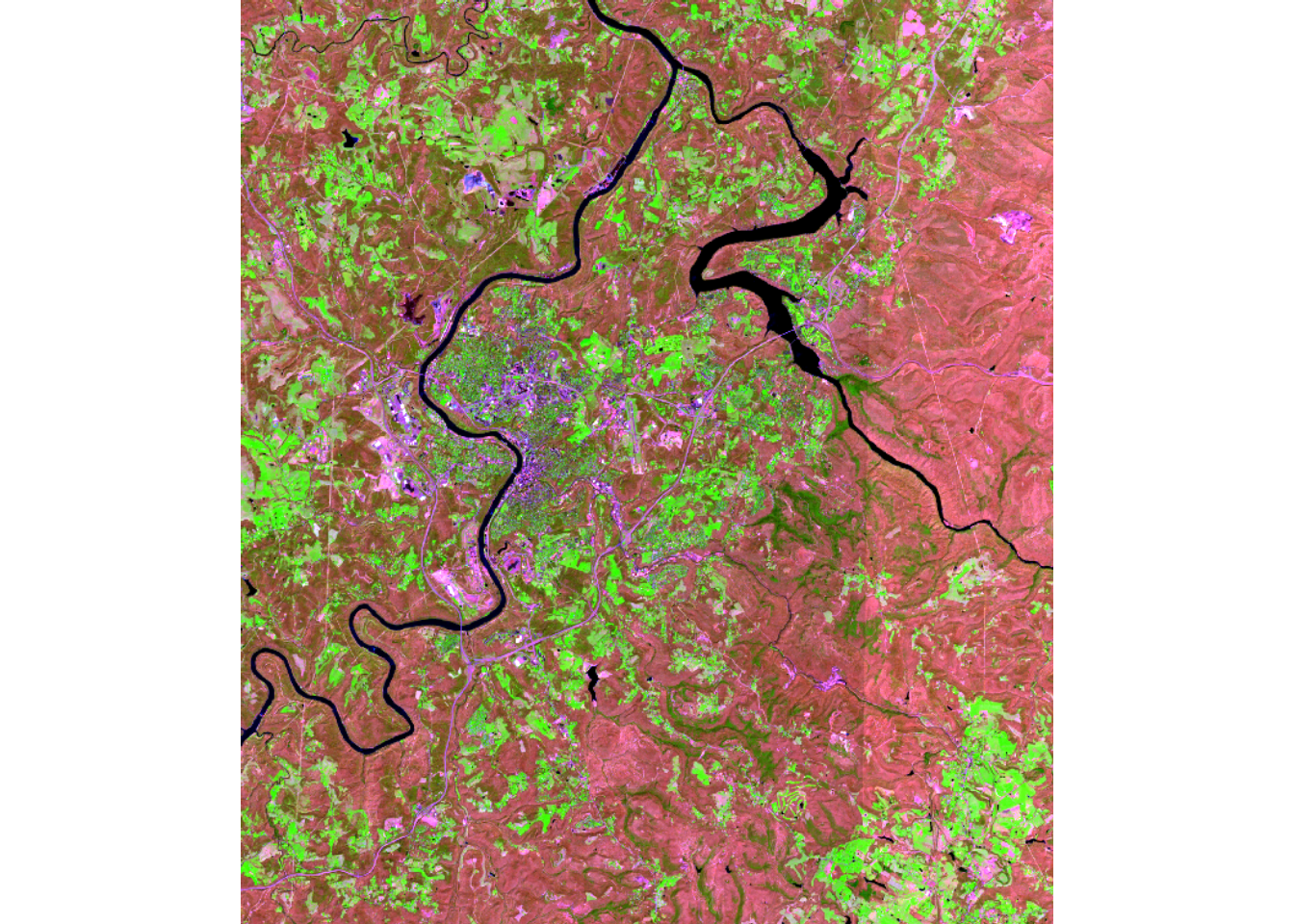
plotRGB(stk,
        r=20,
        g=18,
        b=13, stretch="lin")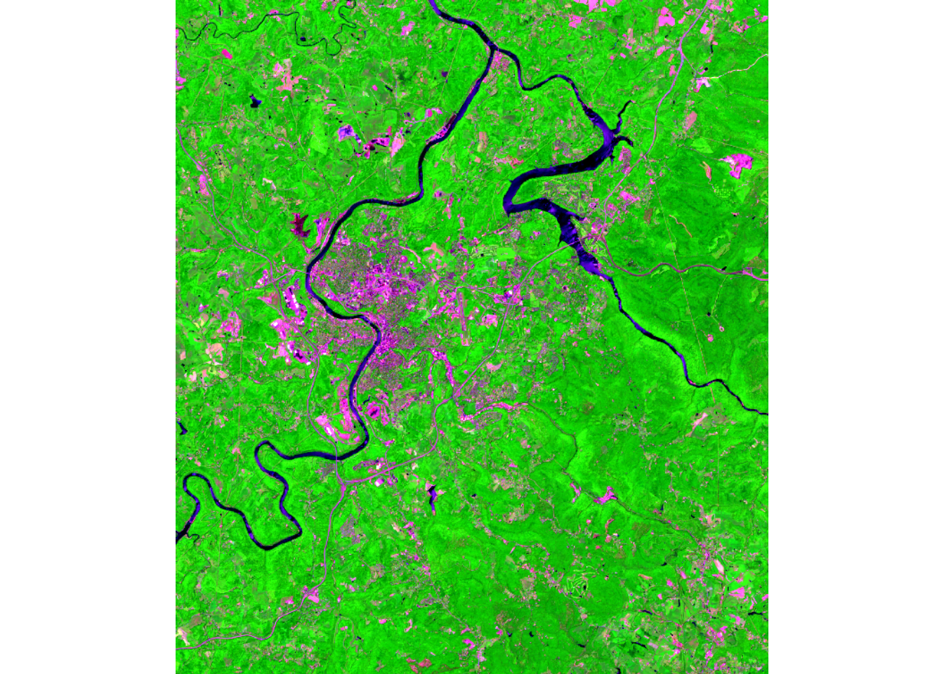
tm_shape(stk$elev)+
tm_raster(style= "cont",
          n=7,
          palette=get_brewer_pal("-Greys", plot=FALSE))+
tm_layout(legend.outside = TRUE)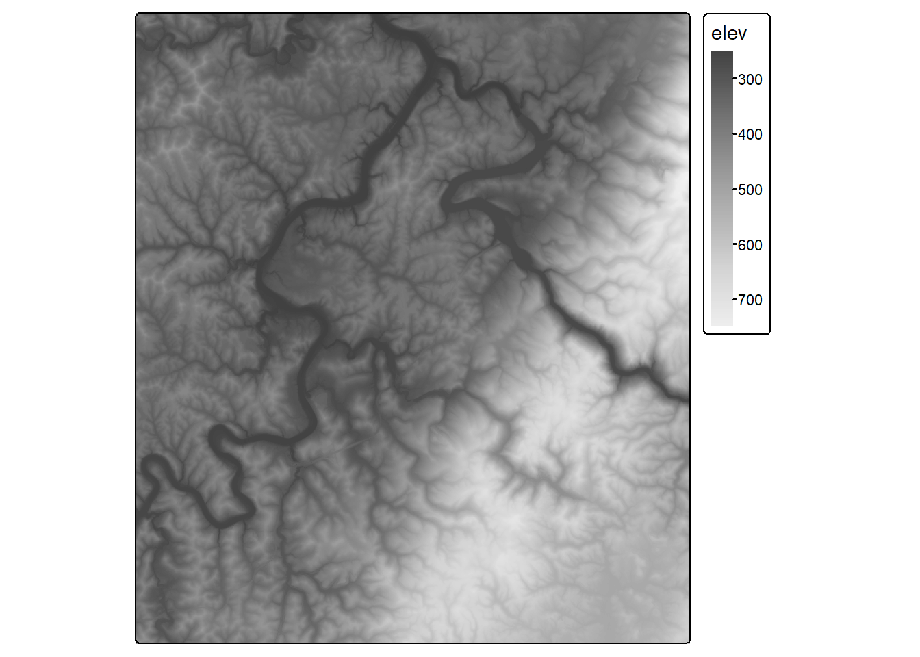
We are now ready to use our trained model to make predictions to each cell in the raster extent. For our demonstration, we use the RF model result. This is undertaken using the following process:
- Extract the cell values into a tibble object, excluding the coordinate information
- use the
predict()function to predict each row in the table with the outputtypeset to"class"so that class labels are returned as opposed to predicted probabilities - Extract a single band from the input raster stack
- Replace the cell values in the extracted band with the generated predictions
- Write the result to disk using the
writeRaster()function from terra as a “.tif” file.
The following code will take some time to execute (~10 minutes). We have provided the output with the chapter files in the data folder so that you do not have to execute the code to display the results.
fldOut <- "gslrData/chpt8/output/"

stkDF <- stk |>
  as.data.frame(stk,
                xy=FALSE,
                na.rm=FALSE) |>
  tibble()

stkPred <- predict(rfModel,
                   new_data = stkDF,
                   type = "class")

clsR <- stk$b1_apr
clsR[] <- stkPred$.pred_class

writeRaster(clsR, str_glue("{fldOut}clsOut.tif"), overwrite=TRUE)
We next read in the result using the rast() function from terra then display it as a categorical raster using tmap. Since these data have been written to disk, they can also be displayed, explored, post-processed, or further analyzed using GIS or remote sensing software.
clsR <- rast(str_glue("{fldPth}clsOut.tif"))

tm_shape(clsR)+
  tm_raster(style= "cat",
            labels = c("Barren",
                       "Conifer Forest",
                       "Deciduous Forest",
                       "Developed",
                       "Grass/Pasture",
                       "Water"),
            palette = c("darkgrey",
                        "darkolivegreen",
                        "darkolivegreen1",
                        "brown4",
                        "goldenrod3",
                        "deepskyblue"),
            title="Land Cover Prediction")+
  tm_layout(legend.outside = TRUE)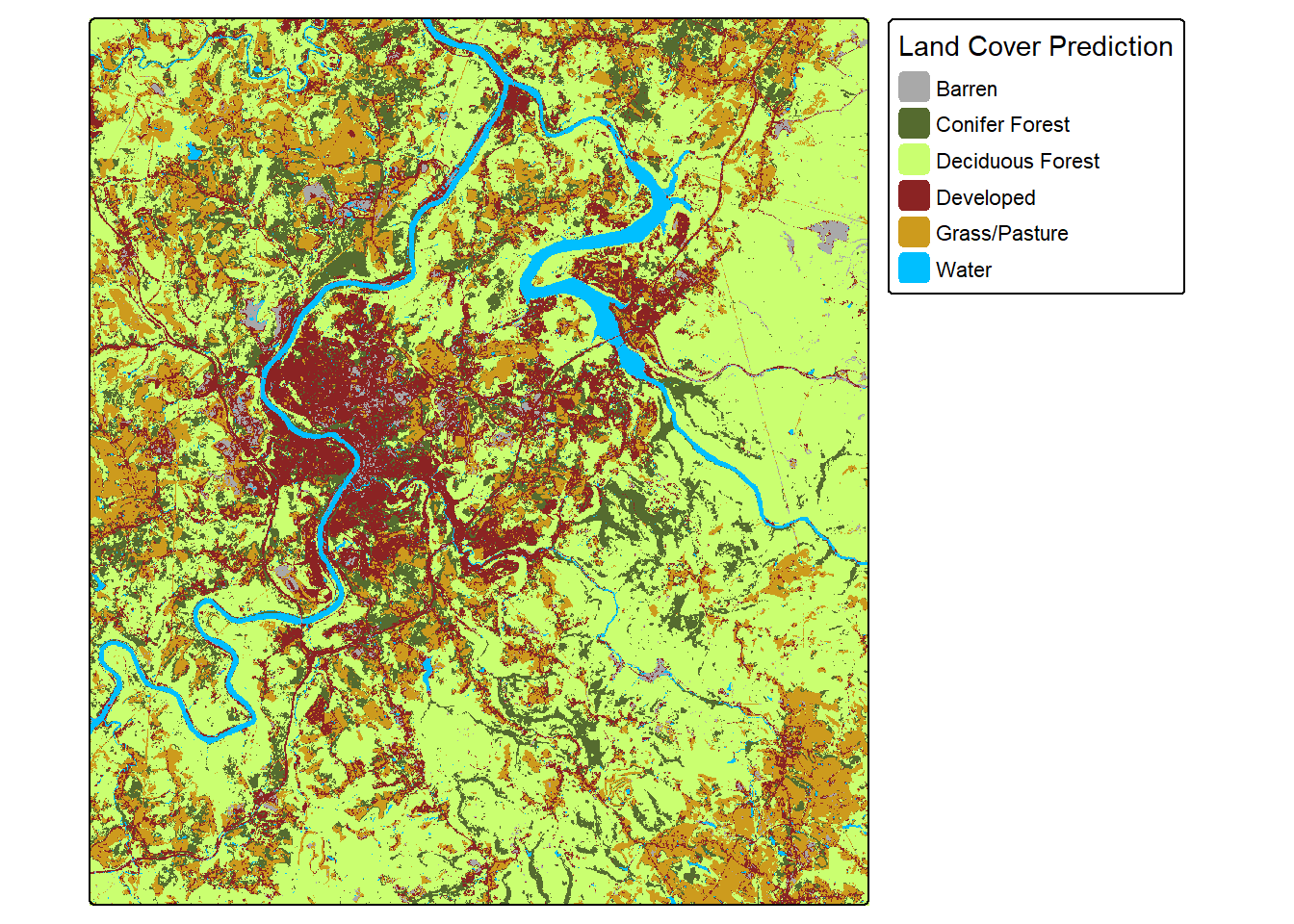
8.2.2.2 Generalize Prediction
The terra package provides tools for generalizing categorical raster data. For example, the sieve() function can be used to remove small, contiguous regions of cells mapped to the same category and replace them with the surrounding class. In the example, we have used a threshold of 1,000 cells; as a result, any region that is smaller than 1,000 cells (10 hectares for this 10 m spatial grain data) will be removed. This is probably too large and will result in too much generalization. However, we wanted to make sure the differences were obvious when displayed. For real applications, this threshold can be selected based on the minimum mapping unit (MMU) defined for the project.
The level of generalization applied should be guided by a defined minimum mapping unit (MMU).
clsRS <- clsR |>
terra::sieve(threshold=1000)tm_shape(clsRS)+
tm_raster(style= "cat",
labels = c("Barren",
"Conifer Forest",
"Deciduous Forest",
"Developed",
"Grass/Pasture",
"Water"),
palette = c("darkgrey",
"darkolivegreen",
"darkolivegreen1",
"brown4",
"goldenrod3",
"deepskyblue"),
title="Land Cover Prediction")+
tm_layout(legend.outside = TRUE)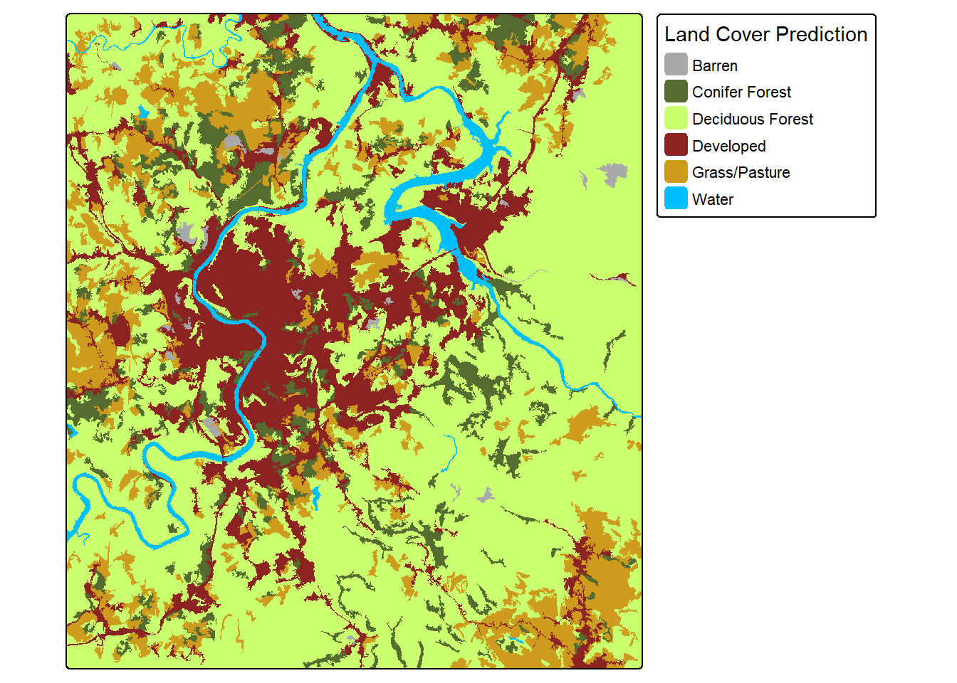
8.3 Workflow 2
We will now augment Workflow 1 to include data preprocessing using the recipes package and accuracy assessment using yardstick. This new workflow is conceptualized in Figure 8.2.
8.3.1 Data Preparation
8.3.1.1 Data Partitioning
As with our first workflow, we begin by reading in the data table, and dplyr is used to (1) convert all character columns to a factor data type, (2) remove unnecessary columns, and (3) drop any row or observation with missing data. We then use stratified random sampling without replacement to select an equal number of samples, 880, per class.
Since we now need to withhold some samples for model assessment, we must partition the data into non-overlapping training and test sets. The initial_split() function from the rsample package can be used to define data partitions. Here, 70% of the data, stratified by the class label, are defined as training samples while the remaining 30% are withheld for model validation as a test set. The training() and testing() functions, also from rsample, are then used to extract the data partitions into separate tibbles.
monD <- read_csv(str_glue("{fldPth}monWFTable.csv")) |>
  mutate_if(is.character, as.factor) |>
  select(-OID_,
         -origComments,
         -CreationDate,
         -Creator,
         -EditDate,
         -Editor) |>
  drop_na()

set.seed(42)
monDStrat <- monD |>
  group_by(lcClass) |>
  sample_n(880,
           replace=FALSE) |>
  ungroup()

set.seed(42)
dataSplit <- monDStrat |>
  initial_split(prop=.7,
                strata=lcClass)

trainD <- training(dataSplit)

testD <- testing(dataSplit)
8.3.1.2 Preprocessing with recipes
The recipes package is used to define data preprocessing pipelines. It is important to adhere to best practices and consider specific model requirements when performing preprocessing. For example, statistics used to normalize or re-scale data should be generated from the training set only as opposed to the full dataset. Including the test data when generating these summary statistics is considered a data leak. Also, some methods require all predictor variables to be on the same scale, specifically those that rely on measures of distance (e.g., SVM and kNN). In contrast, tree-based methods (e.g., decision trees (DTs), RF, and boosted DTs) do not require data to be on a consistent scale.
For our experiment, the image bands are on a different scale than the predictor variables derived from the digital terrain model. So, it would be good to normalize all the variables to a consistent scale. We begin by defining a recipe. Our simple recipe first states the equation for the model, in this case the “lcClass” column is being predicted using all other columns in the tibble. We next indicate that we want to re-scale all predictor variables using step_range() from recipes. This function performs min-max re-scaling to a range of zero to one. Note the use of all_numeric_predictors() to specify which columns to normalize.
This defines the preprocessing pipeline. It can then be prepared using the prep() function, which is also from recipes. This function determines the summary statistics needed to perform the data normalization. To actually undertake the normalization, the preprocessing workflow is applied to both the training and test set tibbles using the bake() function from recipes. If the new_data argument is set to NULL, the training data are processed as opposed to a new dataset.
To check the results, we calculate the new minimum and maximum values for each predictor variable. This confirms that the new range of values is as expected.
myRecipe <- recipe(lcClass ~ ., data = trainD) |>
  step_range(all_numeric_predictors())

myRecipePrep <- prep(myRecipe, training=trainD)

trainDN <- bake(myRecipePrep, new_data=NULL)
testDN  <- bake(myRecipePrep, new_data=testD)

df_numeric <- trainDN |> select(where(is.numeric))
minV   <- map_dbl(df_numeric, min)
maxV <- map_dbl(df_numeric, max)

predStats <- tibble(bands = names(trainDN)[1:23],
                        Minimum = minV,
                        Maximum = maxV)

predStats |> gt()| bands | Minimum | Maximum |
|---|---|---|
| b1_apr | 0 | 1 |
| b2_apr | 0 | 1 |
| b3_apr | 0 | 1 |
| b4_apr | 0 | 1 |
| b5_apr | 0 | 1 |
| b6_apr | 0 | 1 |
| b7_apr | 0 | 1 |
| b8_apr | 0 | 1 |
| b9_apr | 0 | 1 |
| b10_apr | 0 | 1 |
| b1_may | 0 | 1 |
| b2_may | 0 | 1 |
| b3_may | 0 | 1 |
| b4_may | 0 | 1 |
| b5_may | 0 | 1 |
| b6_may | 0 | 1 |
| b7_may | 0 | 1 |
| b8_may | 0 | 1 |
| b9_may | 0 | 1 |
| b10_may | 0 | 1 |
| elev | 0 | 1 |
| slp | 0 | 1 |
| tpi | 0 | 1 |
Here, we have used only a single preprocessing/feature engineering operation to demo the use of the recipes package. However, it is important to note that this package provides a large set of operations that allow for a variety of data manipulations including log, inverse, square root, Box-Cox, and Yeo-Johnson transformations for continuous variables; generation of dummy variables or recoding categorical variables; defining interactions between variables; removing highly correlated, near-zero variance, or incomplete predictor variables; and performing feature reduction using principal component analysis (PCA), kernel PCA, or independent component analysis (ICA). Please see the recipes documentation for a full set of available operations.
8.3.2 Define and Train Models
Now that the data are prepared, we can use parsnips to define models to train. As in the first workflow, we experiment with three different algorithms: RF, SVM, and kNN. We first define the models, which includes specifying hyperparameters and setting the engine and mode. For the RF model, we are use 500 trees in the ensemble and use the default setting for all other hyperparameters, such as the number of random variables to select from at each decision node (mtry). For SVM, we use the kernlab package, a radial basis function (RBF) kernel, and the default values for cost and rbf_sigma. For kNN, we use 11 neighbors.
rfSpec <- rand_forest(trees=500) |>
  set_engine("ranger") |>
  set_mode("classification")

svmSpec <- svm_rbf() |>
  set_engine("kernlab") |>
  set_mode("classification")

knnSpec <- nearest_neighbor(neighbors=11) |>
  set_engine("kknn") |>
  set_mode("classification")
Once models are defined, they are trained using the fit() function from parsnips, which results in a fitted model that can be used to make predictions to new data. This requires defining (1) the dependent variable and set of predictor variables and (2) the training dataset.
rfModel <- rfSpec |>
  fit(lcClass ~.,
      data=trainDN)

svmModel <- svmSpec |>
  fit(lcClass ~.,
      data=trainDN)

knnModel <- knnSpec |>
  fit(lcClass ~.,
      data=trainDN)
8.3.3 Compare and Assess Models
Now that we have trained models, we can assess model performance using the withheld test data. Again, since the test samples are not purely random, this will result in a biased estimate. This is simply a demonstration. The predict() function allows for making predictions to new data using a trained model and requires defining (1) the trained model to use, (2) the new data to infer to, and (3) the type of prediction desired. Since this is a multiclass classification, we set the type argument to "class". For models that also generated class probabilities, type can be set to "prob" to obtain these probabilities. For a regression task, type is commonly set to "numeric". There are other more specific types of predictions that can be obtained, which we do not discuss here.
In the examples below, we are binding the results to the test set tibble so that the predictions and reference labels are stored in the same table.
Once predictions have been obtained for the test set, assessment metrics can be calculated by comparing the predictions to the reference labels. Here, we calculate overall accuracy and macro-averaged, class aggregated F1-score, precision (i.e., user’s accuracy), and recall (i.e., producer’s accuracy). We first define a metric set using the metric_set() function from yardstick. The truth parameter references the reference labels while the estimate parameter references the prediction, which is in the “.pred_class” column in the tables of predictions. We also use mutate() from dplyr to add the name of the algorithm used as a column to the output. Lastly, we merge the metrics for all three models to a single tibble.
Printing the results, we can see that we have obtain a table with four columns. The “.metric” column names the metric calculated while the “.estimator” column notes how it was calculated. Note that "macro" indicates macro- as opposed to micro-averaging. The “.estimate” column provides the metric value while our added “algorithm” column differentiates the different algorithms used. Columns automatically generated by yardstick are commonly prefixed with “.”.
my_metrics <- metric_set(accuracy, f_meas, precision, recall)

rfResult <- rfPred |>
  my_metrics(
    truth = lcClass,
    estimate = .pred_class) |>
  mutate(algorithm = "Random Forest")

svmResult <- svmPred |>
  my_metrics(
    truth = lcClass,
    estimate = .pred_class) |>
  mutate(algorithm = "SVM")

knnResult <- knnPred |>
  my_metrics(
    truth = lcClass,
    estimate = .pred_class) |>
  mutate(algorithm = "kNN")

allResults <- bind_rows(rfResult,
                        svmResult,
                        knnResult)

allResults |> gt()| .metric | .estimator | .estimate | algorithm |
|---|---|---|---|
| accuracy | multiclass | 0.9343434 | Random Forest |
| f_meas | macro | 0.9338952 | Random Forest |
| precision | macro | 0.9351361 | Random Forest |
| recall | macro | 0.9343434 | Random Forest |
| accuracy | multiclass | 0.9299242 | SVM |
| f_meas | macro | 0.9297704 | SVM |
| precision | macro | 0.9311206 | SVM |
| recall | macro | 0.9299242 | SVM |
| accuracy | multiclass | 0.9267677 | kNN |
| f_meas | macro | 0.9265322 | kNN |
| precision | macro | 0.9275525 | kNN |
| recall | macro | 0.9267677 | kNN |
Graphing the results with ggplot2, we can see that the RF algorithm generally provided the best performance as measured using all four assessment metrics. SVM generally outperformed kNN.
metLabs<- c("accuracy" = "Overall Accuracy",
            "f_meas" = "Macro-Averaged F1-Score",
            "precision" = "Macro-Averaged Precision",
            "recall" = "Macro-Averaged Recall")

allResults |>
  ggplot(aes(x=algorithm,
             y=.estimate))+
  geom_point(size=3,
             color="#AC3E31")+
  facet_wrap(vars(.metric),
             labeller = labeller(.metric=metLabs))+
  theme_bw(base_size=14)+
  labs(y="Value",
       x="Algorithm")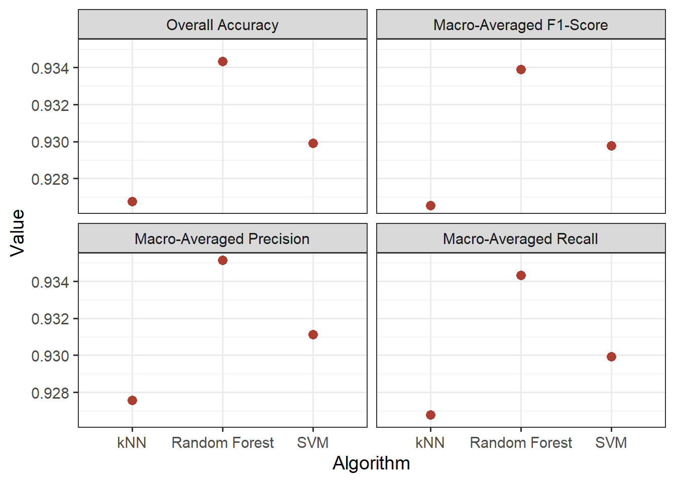
Since the RF algorithm provided the best performance, we can further explore the model using a full confusion matrix, which is generated using the conf_mat() function from yardstick. As is the standard in remote sensing, the columns are defined by the reference labels while the rows are defined by the predicted labels. Generally, we see some confusion between the Barren and Developed classes. This makes sense, since they are spectrally similar. There is also some confusion between Grass and Developed, potentially resulting from residential areas with mixed land cover.
rfPred |>
  conf_mat(truth = lcClass,
           estimate = .pred_class) |>
  print()
Truth
Prediction barren conForest decForest developed grass water
barren 244 0 0 26 4 6
conForest 0 253 2 3 1 2
decForest 1 5 262 4 1 3
developed 10 1 0 217 4 3
grass 6 4 0 13 254 0
water 3 1 0 1 0 2508.4 Concluding Remarks
Now that you have a basic understanding of how the ML workflows is implemented using tidymodels, in the next chapter we will integrate hyperparameter tuning using the rsample, tune, and dials packages. We will also simplify the process using the workflows package. In our final workflow in the next chapter, we will compare different algorithm and preprocessing combinations using workflowsets.
8.5 Questions
- Within the tidymodels metapackage, what is the purpose of the following packages: parsnips, rsample, recipes, and yardstick?
- Explain the purpose of the
set_engine()function within tidymodels. - Explain the purpose of the
set_mode()function within tidymodels. - Explain the purpose of the
recipe(),prep(), andbake()functions from recipes. - Why should
prep()only use the training set as opposed to the full dataset? - What is the purpose of the
costhyperparameter for SVM? - What is the purpose of the
neighborshyperparameter for k-nearest neighbors? - What is the purpose of the baguette package within the tidymodels ecosystem?
8.6 Exercises
This exercise builds upon the data preparation exercise from Chapter 3. You will complete some of the same preprocessing steps then train and compare models using tidymodels.
You have been provided two CSV files: training.csv and test.csv in the exercise folder for the chapter. Both represent data for a object-based image classification. Multiple data layers have been summarized relative to image objects including red, green, blue, and near infrared (NIR) image bands derived from National Agriculture Imagery Program (NAIP) orthophotography; feature heights, return intensity, and topographic slope derived from lidar; density of man-made structures, and density of roads.
Preprocessing
- Read in both tables
- For both tables, complete the following tasks using the tidyverse:
- Extract out the “class” column and all other columns beginning with “Mean” (should result in 16 columns)
- Drop any rows with missing data in any column
- Some of the rows have missing values that contain a very low numeric placeholder value as opposed to
NA(< 1e-30); remove rows that have a value lower then 1e-30 in any numeric column - Remove “Mean” from all column names
- Convert all character columns to factors
- Create a recipe to re-scale all the predictor variables to a range of 0 to 1
- Prepare the recipe using the training data
- Apply the prepared recipe to both the training and test tables
The analysis should result in the following columns (representing mean values from the pixels within the image objects):
- “nDSM”: height above ground in meters
- “Str500”: structure kernel density in 500 m radius window
- “Str250”: structure kernel density in 250 m radius window
- “Str1000”: structure kernel density in 1,000 m radius window
- “Slp”: topographic slope in degrees
- “Roads500”: road kernel density in 500 m radius window
- “Roads250”: road kernel density in 250 m radius window
- “Roads1000”: road kernel density in 1,000 m radius window
- “Red”: red channel
- “NIR”: NIR channel
- “NDVI”: normalized difference vegetation index
- “Int”: first return lidar intensity
- “Green”: green channel
- “Elev”: elevation in meters
- “Blue”: blue channel
- “Class”: classes being differentiated (“barren”, “crop”, “developed”, “forest”, “pasturegrass”, and “water”)
Fit Models
- Specify the following models using tidymodels and parsnips (use defaults for all non-specified settings):
- Random forest with 500 trees
- Support vector machine with an RBF kernel
- k-nearest neighbors with 11 neighbors
- Fit the models using the prepared training set. The “class” column should be predicted by all other columns.
Compare Models
- Use all three trained models to make predictions to the test set.
- Use the predictions and reference labels to calculate overall accuracy, F1-score, recall, and precision for all three models. Use macro-averaging for F1-score, recall, and precision.
- Calculate error matrices for all three models using the test set predictions and reference labels
- Generate a short write-up to compare the performance of the models. Also, discuss general sources of error or confusion in the models. Which classes were most confused or proved most difficult to differentiate?
- Discuss methods you could use to potentially improve the models.