5 Accuracy Assessment
5.1 Topics Covered
- Calculating accuracy assessment metrics using the yardstick package
- Regression metrics (mean square error, root mean square error, mean absolute error, and R-squared)
- Multiclass classification metrics (confusion matrix, overall accuracy, producer’s accuracy/recall, user’s accuracy/precision, F1-score, and macro-averaging)
- Single-threshold binary assessment metrics (confusion matrix, precision, recall, F1-score, negative predictive value, and specificity)
- Multi-threshold binary assessment metrics (receiver operating characteristic curve, precision-recall curve, and area under the curve)
- Map image classification efficacies via the micer package
5.2 Introduction
In order to validate models, it is important to assess their performance on a new dataset. A model that performs well on the training set my be overfit and fail to generalize to new data. In this chapter, we explore assessment metrics for both classification and regression with a focus on the yardstick package, which is part of the tidymodels metapackage. We also explore the micer package, which provides a large set of aggregated and class-level assessment metrics alongside map image classification efficacy (MICE).
5.3 Regression
To experiment with regression metrics, we make use of a hypothetical dataset that includes a known measurement, “truth”, and predictions from three models: “m1”, “m2”, and “m3”. There are a total of 156 samples included.
There are a variety of metrics used to assess regression models. Here, we focus on the most often used measures: mean square error (MSE), root mean square error (RMSE), and mean absolute error (MAE). MSE is simply the mean of the square of the residuals. A residual is the difference between the reference value and predicted value. Since a square is being used, the units of MSE are the square of the units of the variable being predicted. For example, if you are estimating mass in kilograms, the units of MSE would be kg2. RMSE is simply the square root of MSE; as a result, the associated units are the same as the units for the variable being predicted. Lastly, MAE is the mean of the absolute value of the residuals. As with RMSE, the units are the same as those for the dependent variable.
\[ \text{MSE} = \frac{1}{n} \sum_{i=1}^{n} \left( y_i - \hat{y}_i \right)^2 \]
\[ \text{RMSE} = \sqrt{\frac{1}{n} \sum_{i=1}^{n} \left( y_i - \hat{y}_i \right)^2} \]
\[
\text{MAE} = \frac{1}{n} \sum_{i=1}^{n} \left| y_i - \hat{y}_i \right|
\]The code block below shows how to calculate RMSE and MAE using yardstick. Both functions require providing the reference value as the truth argument and the estimated value as the estimate argument. Note also that there are two forms of these functions. For example, RMSE can be calculated using rmse() and rmse_vec(). The “_vec()” version returns the measure as a vector or scalar while the other version returns a tibble where the “.metric” column names the metric, the “.estimator” notes the calculation method, and the “.estimate” column provides the metric value.
[1] 0.37[1] 0.296It is also common to calculate the R-squared measure, which quantifies the proportion of the total variance in the dependent variable explained by the model. The total variance in the model is defined as the sum of the squared differences between each value and the mean value while the total unexplained variance is the sum of squares of the residuals, or difference between the actual and predicted value. Subtracting the residual sum of squares from the total sum of squares provides an estimate of the explained variance. Dividing this result by the total variance yields a value between zero and one where zero indicates that no variance is explained and one indicates that all the variance is explained.
\[ R^2 = 1 - \frac{\sum_{i=1}^{n} \left( y_i - \hat{y}_i \right)^2}{\sum_{i=1}^{n} \left( y_i - \bar{y} \right)^2}, \quad \text{where} \quad \bar{y} = \frac{1}{n} \sum_{i=1}^{n} y_i. \]
The code block below demonstrates how to calculate R-squared using yardstick. For the first model results, the metric suggests that ~77% of the variance in the dependent variable is being explained by the model.
To compare the three models, we now calculate RMSE and R-squared for each then bind the results into a single tibble. Generally, the results suggest that the first model is providing the strongest performance.
rmse1 <- rmse(regIn, truth=truth, estimate=m1)$.estimate |> round(3)
rmse2 <- rmse(regIn, truth=truth, estimate=m2)$.estimate |> round(3)
rmse3 <- rmse(regIn, truth=truth, estimate=m3)$.estimate |> round(3)

rsq1 <- rsq(regIn, truth=truth, estimate=m1)$.estimate |> round(3)
rsq2 <- rsq(regIn, truth=truth, estimate=m2)$.estimate |> round(3)
rsq3 <- rsq(regIn, truth=truth, estimate=m3)$.estimate |> round(3)

regDF <- tibble(Model = c("M1", "M2", "M3"),
                RMSE = c(rmse1, rmse2, rmse3),
                RSqaured = c(rsq1, rsq2, rsq3))

regDF |>gt()| Model | RMSE | RSqaured |
|---|---|---|
| M1 | 0.370 | 0.771 |
| M2 | 0.380 | 0.758 |
| M3 | 0.383 | 0.755 |
The yardstick package supports the calculation of a range of regression metrics including mean signed deviation (MSD), mean percentage error (MPE), concordance correlation coefficient (CCC), ratio of performance to interquartile range (RPIQ), and ratio of performance to deviation (RPD).
5.4 Multiclass Classification
To experiment with accuracy assessment metrics, we will use two example classification results for the EuroSat dataset. We begin by reading in the data. For both results, the predictions are stored in the “pred” column while the reference labels are stored in the “ref” column. Numeric codes are used as opposed to class names, so the columns are read in as a numeric data type; as a result, it is necessary to convert them to factors.
To make our results easier to interpret, we next use the fct_recode() function from the forcats package to recode the numeric codes to more meaningful text labels. Although this is not strictly necessary, we generally find it easier to use class names that are more meaningful and interpretable.
result1$ref <- fct_recode(result1$ref,
                          "AnnCrp" = "0",
                          "Frst" = "1",
                          "HrbVg" = "2",
                          "Highwy" = "3",
                          "Indst" = "4",
                          "Pstr" = "5",
                          "PrmCrp" = "6",
                          "Resid" = "7",
                          "Rvr" = "8",
                          "SL" = "9")

result1$pred <- fct_recode(result1$pred,
                           "AnnCrp" = "0",
                           "Frst" = "1",
                           "HrbVg" = "2",
                           "Highwy" = "3",
                           "Indst" = "4",
                           "Pstr" = "5",
                           "PrmCrp" = "6",
                           "Resid" = "7",
                           "Rvr" = "8",
                           "SL" = "9")

result2$ref <- fct_recode(result2$ref,
                          "AnnCrp" = "0",
                          "Frst" = "1",
                          "HrbVg" = "2",
                          "Highwy" = "3",
                          "Indst" = "4",
                          "Pstr" = "5",
                          "PrmCrp" = "6",
                          "Resid" = "7",
                          "Rvr" = "8",
                          "SL" = "9")

result2$pred <- fct_recode(result2$pred,
                           "AnnCrp" = "0",
                           "Frst" = "1",
                           "HrbVg" = "2",
                           "Highwy" = "3",
                           "Indst" = "4",
                           "Pstr" = "5",
                           "PrmCrp" = "6",
                           "Resid" = "7",
                           "Rvr" = "8",
                           "SL" = "9")
5.4.1 Confusion Matrix
We begin our analysis by creating confusion matrices for each prediction using the conf_mat() function from yardstick. The confusion matrices are formatted such that the columns represent the reference labels and the rows represent the predictions, which is the standard in remote sensing.
Values populating the main diagonal represent correct classifications while those off the diagonal represent incorrect predictions. Off-diagonal counts in a specific column represent omission errors relative to the class associated with that column. For example, in the first classification 6 Annual Crop samples were incorrectly predicted to the Forest class, which represents omission error relative to the Annual Crop class. Counts in off-diagonal cells within a row represent commission errors relative to the class associated with the row. In other word, they represent samples that were incorrectly included in the class associated with the row. For example, 4 Permanent Crop samples were incorrectly included in the Annual Crop class in the first classification.
One of the key benefits of the confusion matrix is the ability to quantify not just the overall error rate but the sources of error, or which classes are most commonly confused.
In remote sensing, we generally configure a confusion matrix such that the columns represent the reference labels and the rows represent the predictions. This may not be the case for all contingency tables, which can lead to calculating user’s and producer’s accuracies incorrectly. So, it is important to make sure the table is formatted as expected.
conf_mat(result1, truth=ref, estimate=pred) Truth
Prediction AnnCrp Frst HrbVg Highwy Indst Pstr PrmCrp Resid Rvr SL
AnnCrp 254 0 3 1 0 0 4 0 0 0
Frst 6 300 12 0 0 4 0 0 0 0
HrbVg 4 0 236 0 1 2 10 1 0 0
Highwy 7 0 3 242 10 1 1 7 1 0
Indst 0 0 1 2 227 0 0 11 0 0
Pstr 6 0 22 0 0 192 6 0 2 0
PrmCrp 22 0 16 2 1 1 226 5 0 0
Resid 0 0 3 1 10 0 1 276 0 0
Rvr 0 0 3 2 1 0 2 0 247 3
SL 1 0 1 0 0 0 0 0 0 356conf_mat(result2, truth=ref, estimate=pred) Truth
Prediction AnnCrp Frst HrbVg Highwy Indst Pstr PrmCrp Resid Rvr SL
AnnCrp 274 0 2 2 0 1 4 0 0 0
Frst 1 289 3 0 0 1 0 0 0 0
HrbVg 5 1 282 2 1 7 16 1 1 0
Highwy 2 0 0 231 5 0 6 3 2 0
Indst 0 0 1 3 236 0 1 1 1 0
Pstr 3 10 2 1 0 188 2 0 1 0
PrmCrp 14 0 4 1 0 3 219 1 0 0
Resid 1 0 2 7 8 0 1 294 0 0
Rvr 0 0 4 3 0 0 1 0 243 1
SL 0 0 0 0 0 0 0 0 2 358It is important to distinguish between a sample confusion matrix and an estimated population confusion matrix. The population confusion matrix is the confusion matrix for the entire map, and generally is the statistical information of interest. However, it is usually impractical to identify the correct value of every pixel in the population, and thus most confusion matrices are based on a sample, from which the population confusion matrix is estimated. The sample confusion matrix itself is only a direct estimate of the population confusion matrix if the sampling from the map was based on simple random sampling. Note that if stratified sampling is used, with sampling probabilities that vary by class (e.g., to produce a “balanced” dataset), then this information needs to be incorporated in the analysis for estimating the population confusion matrix. One way of understanding the difference between the sample and estimated population confusion matrix is to consider that only in the estimated population confusion matrix is the sum of the values in the table for a particular reference class (i.e. a column total) an estimate of the proportion of that class within the landscape being mapped.
5.4.2 Multiclass Assessment Metrics
A variety of assessment metrics can be generated from the confusion matrix. For each class, it is possible to calculate measures associated with omission and commission errors. Producer’s accuracy or recall for a class is calculated by dividing the correct count by the column total while user’s accuracy or precision is calculated by dividing the correct count by the row total. Note that it is common to report these metrics as proportions instead of percentages.
\[ \text{Recall}_i = \frac{C_{ii}}{\sum_{j=1}^{k} C_{ij}} \]
\[ \text{Precision}_i = \frac{C_{ii}}{\sum_{j=1}^{k} C_{ji}} \]
To summarize:
- Producer’s Accuracy = Recall = 1 - Omission Error
- User’s Accuracy = Precision = 1 - Commission Error
The overall accuracy is simply the count correct divided by the sum of the entire table. It is sometimes reported as a proportion and sometimes as a percentage.
\[ \text{Accuracy} = \frac{\sum_{i=1}^{k} C_{ii}}{\sum_{i=1}^{k} \sum_{j=1}^{k} C_{ij}} \]
It is possible to aggregate class-level producer’s accuracy/recall or class-level user’s accuracy/precision to a single metric using micro- or macro-averaging. Micro-averaging is actually equivalent to overall accuracy, so it is not necessary to calculate and report additional metrics calculated using this method. Macro-averaging is conducted by calculating the metrics separately for each class then taking the average such that each class has equal weight in the aggregated metric regardless of the relative abundances of the classes in the dataset or landscape of interest. If desired, it is also possible to incorporate class weights such that each class is not equally weighted.
\[ \text{Macro-Averaged Class Aggregated Precision ()} = \frac{1}{k} \sum_{i=1}^{k} \text{Precision}_i \]
\[ \text{Macro-Averaged Class Aggregated Recall} = \frac{1}{k} \sum_{i=1}^{k} \text{Recall}_i \]
Lastly, the F1-score is the harmonic mean of the precision and recall for a class. For macro-averaging, the metric is calculated separately for each class then averaged. Note that this metric is perfectly correlated with the intersection-over-union (IoU) metric, so it is not necessary to calculate both metrics.
\[ \text{Macro-Averaged Class Aggregated F1-Score} = \frac{1}{k} \sum_{i=1}^{k} \left( 2 \times \frac{\text{Precision}_i \times \text{Recall}_i}{\text{Precision}_i + \text{Recall}_i} \right) \]
The code below demonstrates how to calculate these metrics using the yardstick package. The truth argument references the column associated with the reference label, in this case the “ref” column, while the estimate argument references the prediction, in this case the “pred” column. These functions return tibbles as opposed to single values. As noted above for the regression metrics, the “.metric” column names the metric, the “.estimator” column notes the calculation method (for example, micro- vs. macro-averaging), and the “.estimate” column provides the metric value. In the code, we are extracting out only the value.
Lastly, we merge the results into a single tibble and print the results, which suggest that the second model, “Result 2”, is generally outperforming the other model for this task.
Since micro-averaged, class aggregated precision, recall, and F1-score are equivalent to each other and also to overall accuracy, there is no need to report these when overall accuracy is reported.
acc1 <- accuracy(result1, truth=ref, estimate=pred)$.estimate |> round(3)
recall1 <- recall(result1, truth=ref, estimate=pred, estimator="macro")$.estimate |> round(3)
precision1 <- precision(result1, truth=ref, estimate=pred, estimator="macro")$.estimate |> round(3)
fscore1 <- f_meas(result1, truth=ref, estimate=pred, estimator="macro")$.estimate |> round(3)

acc2 <- accuracy(result2, truth=ref, estimate=pred)$.estimate |> round(3)
recall2 <- recall(result2, truth=ref, estimate=pred, estimator="macro")$.estimate |> round(3)
precision2 <- precision(result2, truth=ref, estimate=pred, estimator="macro")$.estimate |> round(3)
fscore2 <- f_meas(result2, truth=ref, estimate=pred, estimator="macro")$.estimate |> round(3)

metricsDF <- data.frame(Model = c("Result 1", "Result 2"),
                        Accuracy=c(acc1, acc2),
                        F1Score = c(fscore1,fscore2),
                        Precision = c(precision1, precision2),
                        Recall = c(recall1, recall2))
metricsDF |> gt()| Model | Accuracy | F1Score | Precision | Recall |
|---|---|---|---|---|
| Result 1 | 0.926 | 0.923 | 0.923 | 0.927 |
| Result 2 | 0.947 | 0.945 | 0.945 | 0.945 |
Also as noted above, there are also versions of these functions that accept a vector of reference labels and a vector of predictions and return just the metric value as opposed to a tibble. These functions have the same name but are suffixed with “_vec”. These functions are demonstrated below.
accuracy_vec(truth=result1$ref, estimate=result1$pred) |> round(3)[1] 0.926recall_vec(truth=result1$ref, estimate=result1$pred, estimator="macro") |> round(3)[1] 0.927precision_vec(truth=result1$ref, estimate=result1$pred, estimator="macro") |> round(3)[1] 0.923f_meas_vec(truth=result1$ref, estimate=result1$pred, estimator="macro") |> round(3)[1] 0.923accuracy_vec(truth=result1$ref, estimate=result2$pred) |> round(3)[1] 0.947recall_vec(truth=result1$ref, estimate=result2$pred, estimator="macro") |> round(3)[1] 0.945precision_vec(truth=result1$ref, estimate=result2$pred, estimator="macro") |> round(3)[1] 0.945f_meas_vec(truth=result1$ref, estimate=result2$pred, estimator="macro") |> round(3)[1] 0.945Several other classification metrics are provide by yardstick including Matthews correlation coefficient (MCC) and the Kappa statistic. However, we generally discourage the use of Kappa.
5.5 Binary Classification
Since it is common to use different terminology for a binary classification with a positive, presence, or true case and a negative, absence, or false class, we will now discuss a binary classification problem.
5.5.1 Single-Threshold
Single-threshold metrics are those that are calculated using the “hard” classification based on a specific decision threshold as opposed to the predicted probability of class membership, sometimes referred to as a “soft” label or prediction. For example, a sample with a predicted probability greater than 0.5 of occurring in the positive case may be coded to “positive” while samples that do not meet this criteria are coded to “negative”. Generally, the user can specify the desired threshold. At this specific threshold each sample can be labelled as one of the following:
- True Positive (TP): referenced to the positive class and correctly labeled as positive
- True Negative (TN): referenced to the negative class and correctly labeled as negative
- False Positive (FP): referenced to the negative class and incorrectly labeled as positive (commission error relative to the positive class and omission error relative to the negative class)
- False Negative (FN): referenced to the positive class and incorrectly labeled as negative (omission error relative to the positive class and commission error relative to the negative class)
From the count of TP, TN, FP, and FN samples, several metrics can be calculated. Recall, also referred to as sensitivity, considers the omission error relative to the positive case. It is equivalent to 1 - positive case omission error or the positive case producer’s accuracy. Precision quantifies commission error relative to the positive case and is equivalent to 1 - positive case commission error or the positive case user’s accuracy. Negative predictive value (NPV) is equivalent to 1 - negative case commission error or the user’s accuracy for the negative case while specificity is equivalent to 1 - negative case omission error or producer’s accuracy for the negative case.
\[ \text{Recall} = \frac{TP}{TP + FN} \]
\[ \text{Precision} = \frac{TP}{TP + FP} \]
\[ \text{Negative Predictive Value (NPV)} = \frac{TN}{TN + FN} \]
\[ \text{Specificity} = \frac{TN}{TN + FP} \]
As noted above, the F1-score is the harmonic mean of precision and recall. It is generally only calculated for the positive case as opposed to averaging across the positive and negative case for a binary classification problem. Note that overall accuracy for a binary classification is the same as that for a multiclass classification: the total correct, TP + TN, divided by the total number of samples.
\[ \text{F1 Score} = 2 \times \frac{\text{Precision} \times \text{Recall}}{\text{Precision} + \text{Recall}} = \frac{2 \times TP}{2 \times TP + FP + FN} \]
To experiment with a binary classification result, we will use a dataset generated by the authors and associated with the problem of predicting whether or not a location is a landslide based on topographic characteristics. In the code block below, we read in the data and recode the labels to “Class 1” and “Class 2”. In this case, “Class 2” represents slope failures while “Class 1” represents not slope failures or the background class. When calculating binary metrics, it is important to set the estimator argument to "binary" and specify which class represents the positive case. Since “Class 2” represents the positive case for this problem, we set the event-level argument to "second". We also generate a confusion matrix using the conf_mat() function.
For the landslide case, “Class 2”, there are more FPs in comparison to FNs. In other words, precision (~0.85) is lower than recall (~0.91).
biIn <- read_csv(str_glue("{fldPth}binary_data.csv"))
names(biIn) <- c("truth", "predicted", "Class1", "Class2")
biIn$truth <- fct_recode(biIn$truth,
                         "Class1" = "not",
                         "Class2" = "slopeD")
biIn$predicted <- fct_recode(biIn$predicted,
                             "Class1" = "not",
                             "Class2" = "slopeD")

yardstick::recall_vec(truth=biIn$truth, estimator="binary", event_level="second", estimate=biIn$predicted) |> round(3)
[1] 0.906yardstick::precision_vec(truth=biIn$truth, estimator="binary", event_level="second", estimate=biIn$predicted) |> round(3)[1] 0.853yardstick::npv_vec(truth=biIn$truth, estimator="binary", event_level="second", estimate=biIn$predicted) |> round(3)[1] 0.9yardstick::spec_vec(truth=biIn$truth, estimator="binary", event_level="second", estimate=biIn$predicted) |> round(3)[1] 0.844yardstick::f_meas_vec(truth=biIn$truth, estimator="binary", event_level="second", estimate=biIn$predicted) |> round(3)[1] 0.879conf_mat(data=biIn, truth=truth, estimate=predicted) Truth
Prediction Class1 Class2
Class1 422 47
Class2 78 4535.5.2 Multi-Threshold
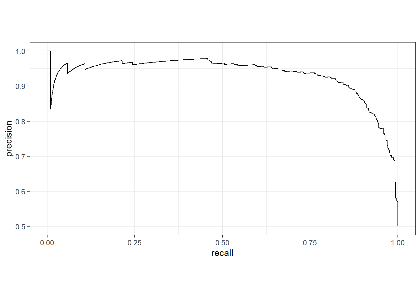
It is also possible to generate metrics using multiple thresholds calculated from the “soft” predictions as opposed to a single threshold. Two common methods are the receiver operating characteristic curve (ROC curve) and precision-recall curve (PR curve). These curves can be aggregated to a single metric by integrating the area under the curve. These measures are called areas under the ROC curve (AUCROC) and area under the P-R curve (AUCPR).
The AUC curve considers sensitivity (i.e., recall) and specificity at multiple thresholds. In other words, in considers 1 - omission error relative to the positive and negative case, respectively. Omission errors are not impacted by class imbalanced, so the curve and associated AUCROC metric will not change as class proportions change. Since both sensitivity and specificity are scaled from zero to one, the maximum possible area under the curve is one.
The PR curves considers precision and recall. In other words it considers 1 - commission and 1 - omission error relative to the positive case at multiple thresholds. Precision is impacted by the the relative class proportions. As a result, PR curves and the associated AUCPR metric will vary as class proportions change. PR curves are generally considered more meaningful than ROC curves when their is significant class imbalance or when the positive or background case make up a much smaller or much larger percentage of the landscape. As with ROC curves, and since both precision and recall are scaled from zero to one, the maximum possible area under the curve is one.
Both ROC and PR curves and associated metrics can be calculated for multi-class problems. However, that is not demonstrated here.
The code below generates an ROC curve using the binary classification results. Note that this requires providing the “hard” correct label as the truth argument and the predicted probability for the positive case. It is also important to specify which label represents the positive case using the event_level argument.
roc_curve(biIn, Class2, truth=truth, event_level="second") |>
  ggplot(aes(x = 1 - specificity, y = sensitivity)) +
  geom_path() +
  geom_abline(lty = 3) +
  coord_equal() +
  theme_bw()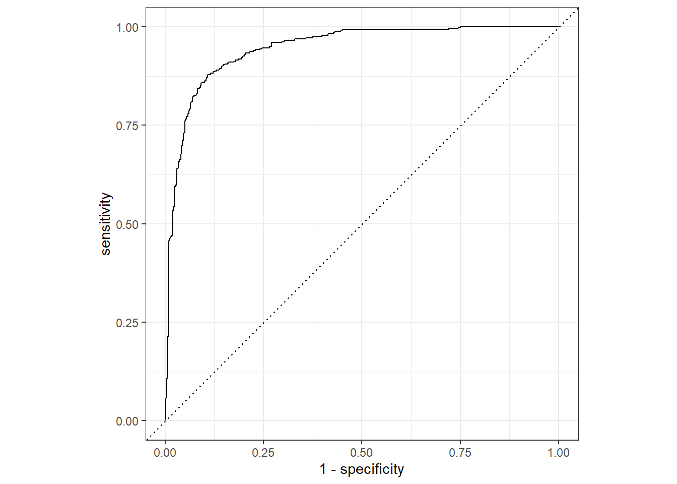
The AUCROC is calculated using the roc_auc() function. For these data, we obtain an AUCROC of 0.945. Note that this measure is generally interpreted like a US university grading scale:
- .9 to 1 = A (excellent)
- .8 to .9 = B (good)
- .7 to .8 = C (acceptable)
- <.7 = D/F (unacceptable)
However, an acceptable AUCROC will depend on the specific use case. Also, a AUCROC of 0.5 is generally interpreted as a model that is performing no better than a random guess.
| .metric | .estimator | .estimate |
|---|---|---|
| roc_auc | binary | 0.945172 |
The next two cold blocks demonstrate the generation of a PR curve and the associated AUCPR metric. The syntax is very similar to that for the ROC curve and AUCROC metric, and AUCPR values are often interpreted similarly to AUCROC, like a college grading scale, other than the consideration that changes in relative class proportions will change the results.
5.6 Map Image Classification Efficacies (MICE)
MICE adjusts the accuracy rate relative to a random classification baseline. Only the proportions from the reference labels are considered, as opposed to the proportions from the reference and predictions, as is the case for the Kappa statistic. Due to documented issues with the Kappa statistic, its use in remote sensing and thematic map accuracy assessment is being discouraged. This metric was introduced in the following papers:
Shao, G., Tang, L. and Zhang, H., 2021. Introducing image classification efficacies. IEEE Access, 9, pp.134809-134816.
Tang, L., Shao, J., Pang, S., Wang, Y., Maxwell, A., Hu, X., Gao, Z., Lan, T. and Shao, G., 2024. Bolstering Performance Evaluation of Image Segmentation Models with Efficacy Metrics in the Absence of a Gold Standard. IEEE Transactions on Geoscience and Remote Sensing.
It can be calculated using the micer package. The metrics calculated depend on whether the problem is framed as a multiclass or binary classification. Multiclass must be used when more than two classes are differentiated. If two classes are differentiated, binary should be used if there is a clear positive, presence, or foreground class and a clear negative, absence, or background class. If this is not the case, multiclass mode is more meaningful.
The mice() function is used to calculate a set of metrics by providing vectors or a data frame/tibble containing columns of reference and predicted class labels. Alternatively, the miceCM() function can be used to calculate the metrics from a confusion matrix table where the columns represent the correct labels and the rows represent the predicted labels.
Results are returned as a list object. For a multiclass classification, the following objects are returned:
-
Mappings= class names -
confusionMatrix= confusion matrix where columns represent the reference data and rows represent the classification result -
referenceCounts= count of samples in each reference class -
predictionCounts= count of predictions in each class -
overallAccuracy= overall accuracy -
MICE= map image classification efficacy -
usersAccuracies= class-level user’s accuracies (1 - commission error) -
CTBICEs= classification-total-based image classification efficacies (adjusted user’s accuracies) -
producersAccuracies= class-level producer’s accuracies (1 - omission error) -
RTBICEs= reference-total-based image classification efficacies (adjusted producer’s accuracies) -
F1Scores= class-level harmonic means of user’s and producer’s accuracies -
F1Efficacies= F1-score efficacies -
macroPA= class-aggregated, macro-averaged producer’s accuracy -
macroRTBICE= class-aggregated, macro-averaged reference-total-based image classification efficacy -
macroUA= class-aggregated, macro-averaged user’s accuracy -
macroCTBICE= class-aggregated, macro-averaged classification-total-based image classification efficacy -
macroF1= class-aggregated, macro-averaged F1-score -
macroF1Efficacy= class-aggregated, macro-averaged F1 efficacy
The results are demonstrated below for our multiclass example.
mice(result1$ref,
     result2$pred,
     multiclass=TRUE)
$Mappings
[1] "AnnCrp" "Frst" "HrbVg" "Highwy" "Indst" "Pstr" "PrmCrp" "Resid"
[9] "Rvr" "SL"
$confusionMatrix
Reference
Predicted AnnCrp Frst HrbVg Highwy Indst Pstr PrmCrp Resid Rvr SL
AnnCrp 274 0 2 2 0 1 4 0 0 0
Frst 1 289 3 0 0 1 0 0 0 0
HrbVg 5 1 282 2 1 7 16 1 1 0
Highwy 2 0 0 231 5 0 6 3 2 0
Indst 0 0 1 3 236 0 1 1 1 0
Pstr 3 10 2 1 0 188 2 0 1 0
PrmCrp 14 0 4 1 0 3 219 1 0 0
Resid 1 0 2 7 8 0 1 294 0 0
Rvr 0 0 4 3 0 0 1 0 243 1
SL 0 0 0 0 0 0 0 0 2 358
$referenceCounts
AnnCrp Frst HrbVg Highwy Indst Pstr PrmCrp Resid Rvr SL
300 300 300 250 250 200 250 300 250 359
$predictionCounts
AnnCrp Frst HrbVg Highwy Indst Pstr PrmCrp Resid Rvr SL
283 294 316 249 243 207 242 313 252 360
$overallAccuracy
[1] 0.9474447
$MICE
[1] 0.9414529
$usersAccuracies
AnnCrp Frst HrbVg Highwy Indst Pstr PrmCrp Resid
0.9681978 0.9829932 0.8924050 0.9277108 0.9711934 0.9082125 0.9049586 0.9392971
Rvr SL
0.9642857 0.9944444
$CTBICEs
AnnCrp Frst HrbVg Highwy Indst Pstr PrmCrp Resid
0.9643176 0.9809181 0.8792770 0.9205069 0.9683227 0.9010378 0.8954874 0.9318905
Rvr SL
0.9607266 0.9936133
$producersAccuracies
AnnCrp Frst HrbVg Highwy Indst Pstr PrmCrp Resid
0.9133333 0.9633333 0.9400000 0.9240000 0.9440000 0.9400000 0.8760000 0.9800000
Rvr SL
0.9720000 0.9972145
$RTBICEs
AnnCrp Frst HrbVg Highwy Indst Pstr PrmCrp Resid
0.9027588 0.9588595 0.9326792 0.9164263 0.9384194 0.9353099 0.8636429 0.9775597
Rvr SL
0.9692097 0.9967977
$f1Scores
AnnCrp Frst HrbVg Highwy Indst Pstr PrmCrp Resid
0.9399657 0.9730639 0.9155844 0.9258517 0.9574036 0.9238329 0.8902439 0.9592169
Rvr SL
0.9681275 0.9958275
$f1Efficacies
AnnCrp Frst HrbVg Highwy Indst Pstr PrmCrp Resid
0.9325234 0.9697634 0.9051911 0.9184621 0.9531365 0.9178540 0.8792770 0.9541790
Rvr SL
0.9649495 0.9952030
$macroPA
[1] 0.9449881
$macroRTBUCE
[1] 0.9391663
$macroUA
[1] 0.9453699
$macroCTBICE
[1] 0.9396098
$macroF1
[1] 0.9451789
$macroF1Efficacy
[1] 0.939388For a binary classification, the following objects are returned within a list object:
-
Mappings= class names -
confusionMatrix= confusion matrix where columns represent the reference data and rows represent the classification result -
referenceCounts= count of samples in each reference class -
predictionCounts= count of predictions in each class -
positiveCase= name or mapping for the positive case -
overallAccuracy= overall accuracy -
MICE= map image classification efficacy -
Precision= precision (1 - commission error relative to positive case) -
precisionEfficacy= precision efficacy -
NPV= negative predictive value (1 - commission error relative to negative case) -
npvEfficacy= negative predictive value efficacy -
Recall= recall (1 - omission error relative to positive case) -
recallEfficacy= recall efficacy -
specificity= specificity (1 - omission error relative to negative case) -
specificityEfficacy= specificity efficacy -
f1Score= harmonic mean of precision and recall -
f1Efficacy= F1-score efficacy
The results are demonstrated below for our binary example.
mice(biIn$truth,
     biIn$predicted,
     multiclass=FALSE,
     positiveIndex=1)
$Mappings
[1] "Class1" "Class2"
$confusionMatrix
Reference
Predicted Class1 Class2
Class1 422 47
Class2 78 453
$referenceCounts
Class1 Class2
500 500
$predictionCounts
Class1 Class2
469 531
$positiveCase
[1] "Class1"
$overallAccuracy
[1] 0.875
$mice
[1] 0.74999
$Precision
[1] 0.8997868
$precisionEfficacy
[1] 0.7995695
$NPV
[1] 0.8531073
$npvEfficacy
[1] 0.7062088
$Recall
[1] 0.844
$recallEfficacy
[1] 0.6879937
$Specificity
[1] 0.906
$specificityEfficicacy
[1] 0.8119962
$f1Score
[1] 0.871001
$f1ScoreEfficacy
[1] 0.7395972It is also possible to estimate confidence intervals for the aggregated metrics using the miceCI() function and using a bootstrap method. In the example below, 1,000 replicated are generated, 70% of the data with replacement are used in each sample, and a 95% confidence interval is estimated. For all the aggregated metric, the mean, median, and lower and upper confidence interval values are estimated. The example below generates the results for our example multiclass classification problem.
ciResultsMC <- miceCI(rep=1000,
                      frac=.7,
                      result1$ref,
                      result1$pred,
                      lowPercentile=0.025,
                      highPercentile=0.975,
                      multiclass=TRUE)

ciResultsMC |> gt()| metric | mean | median | low.ci | high.ci |
|---|---|---|---|---|
| overallAccuracy | 0.9260989 | 0.9259451 | 0.9145520 | 0.9373382 |
| MICE | 0.9176343 | 0.9174724 | 0.9047982 | 0.9301307 |
| macroPA | 0.9269741 | 0.9269344 | 0.9157374 | 0.9385132 |
| macroRTBUCE | 0.9187337 | 0.9186983 | 0.9064102 | 0.9313971 |
| macroUA | 0.9228861 | 0.9227111 | 0.9112341 | 0.9344061 |
| macroCTBICE | 0.9150543 | 0.9148550 | 0.9023634 | 0.9278416 |
| macroF1 | 0.9249245 | 0.9247341 | 0.9136142 | 0.9359322 |
| macroF1Efficacy | 0.9168892 | 0.9167383 | 0.9042231 | 0.9292069 |
Lastly, it is possible to statistically compare two classifications using a paired t-test and bootstrapping to estimate the sample distribution. This is implemented with the miceCompare() function. It is based on a method outlined in Chapter 11 of Tidy Modeling in R.
For the multiclass classification, statistical difference between the model results is assumed using a p-value of 0.05 or a 95% confidence interval (p-value = < 2.2e-16).
miceCompare(ref=result1$ref,
            result1=result1$pred,
            result2=result2$pred,
            reps=1000,
            frac=.7)
    Paired t-test

data:  resultsDF$mice1 and resultsDF$mice2
t = -109.34, df = 999, p-value < 2.2e-16
alternative hypothesis: true mean difference is not equal to 0
95 percent confidence interval:
 -0.02382740 -0.02298724
sample estimates:
mean difference
    -0.02340732
5.7 Concluding Remarks
This chapter concludes the first section of the text. We will now move on to explore different supervised learning algorithms. Throughout Section 2 and 3 of the text, we will implement the accuracy assessment methods and metrics introduced in this chapter.
5.8 Questions
- For the yardstick package, explain the difference between the regular and “_vec” version of a metric (for example,
recall()vs.recall_vec()). - Explain the terms true positive, true negative, false positive, and false negative using an example.
- Explain the difference between omission and commission error using an example.
- If the relative proportion of classes in a multiclass classification change, will class-level recall change? Explain your reasoning.
- If the relative proportion of classes in a multiclass classification change, will class-level precision change? Explain your reasoning.
- Explain the difference between micro- and macro-averaging methods when calculating a single, aggregated metric from class-level metrics.
- Explain the difference between a receiver operating characteristic (ROC) curve and a precision-recall (PR) curve.
- Explain the concordance correlation coefficient (CCC) and how it is different from the Pearson correlation coefficient.
5.9 Exercises
Multiclass Classification
You have been provided with accuracy assessment results for a land cover mapping project for the entire state of West Virginia as a point layer (chpt5.gpkg/multiClassWV) in the exercise folder for the chapter. The “GrndTruth” column represents the reference labels while the “pred” column represents the predictions. Complete the following tasks:
- Read in the point features
- Use dplyr to re-code the class indices for both the “GrndTruth” and “pred” columns as follows:
- 1 = “Forest”
- 2 = “LowVeg”
- 3 = “Barren”
- 4 = “Water”
- 5 = “Impervious”
- 6 = “Mix Dev”
- Make sure all character columns are treated as factors
- Generate a confusion matrix using yardstick
- Calculate overall accuracy using yardstick
- Calculate class-aggregated, macro-average recall, precision, and F1-score using yardstick
- Write a paragraph describing the assessment results. Which classes were most confused? What classes were generally well differentiated?
Binary Classification
You have been provided with accuracy assessment results for the extraction of surface mine disturbance from historic topographic maps where two classes are differentiated: “Background” and “Mine”. “Mine” is considered the positive case while “Background” is the negative, background, or absence case. Three files have been provided in the exercise folder for the chapter:
- chpt5.gpkg/valPnts: point location at which to perform validation
- topo_pred2.tif: raster of predictions (0 = “Background”; 255 = “Mine”)
- topo_ref.tif: raster of reference labels (0 = “Background”; 255 = “Mine”)
Perform the following tasks:
- Extract the prediction and reference indices to the point locations
- In the resulting table, re-code the numeric codes to class names
- Make sure all character columns are treated as factors
- Calculate a confusion matrix using yardstick
- Calculate overall accuracy, precision, recall, and F1-score using yardstick (make sure the correct class is treated as the positive case)
- Write a paragraph describing the sources of error in the results. Make sure to distinguish between commission and omission errors.