14 UNet Archiecture (Semantic Segmentation)
14.1 Topics Covered
- Subclass
nn_module()to generate model components - Generate a UNet architecture from scratch by subclass
nn_module() - Incorporate a scene labeling architecture as the encoder component of UNet
14.2 Introduction
The last three chapters focused on scene classification or scene labeling where the entire image extent is labeled to a single class. For the EuroSat dataset specifically, each 64-by-64 pixel image was labeled to one of ten pre-defined classes. The next three chapters explore semantic segmentation where each pixel is classified separately. One example use case of such methods is land cover classification, such as the data provided by the National Land Cover Database. In this chapter, we build the UNet architecture from scratch using torch. In the next two chapters, we implement geospatial semantic segmentation using the geodl package, which builds on torch, luz, and terra. The following is the original citation for UNet:
Ronneberger O, Fischer P, Brox T. U-net: Convolutional networks for biomedical image segmentation. International Conference on Medical image computing and computer-assisted intervention. Springer; 2015. pp. 234–241.
We have chosen to focus on UNet here since it is a fairly intuitive and widely used architecture. Many subsequent architectures have built upon it or further expanded it. UNet can be thought of as not a single architecture but a general framework with some commonalities being the use of an encoder-decoder design and skip connections.
Figure 14.1(a) conceptualizes a simple UNet, similar to the one introduced by Ronneberger et al. (2015). The goal of the encoder is to learn spatial abstractions of the data at varying spatial scales. Although different architectures can be used for each block, a double-convolution configuration, as conceptualized in Figure 14.1(b), is commonly used. This consists of two 2D convolutional layers each with an associated 2D batch normalization and rectified linear unit (ReLU) activation. In the architecture we build here, each encoder, decoder, and the bottleneck block use this configuration. The convolution layers use 3x3 kernels with a padding of one to maintain the array size in the spatial dimensions. In the encoder, each block is separated by a 2D max pooling operation that uses a 2x2 window with a stride of two that decreases the spatial resolution of its input by half. The goal is to decrease the size of the feature maps in order to allow for learning patterns at different spatial resolutions or scales. The bottleneck represents the stage of the architecture where the array has the smallest spatial resolution but the highest degree of semantic information has been captured. In our example architecture with four encoder blocks, the spatial resolution has been decreased by a factor of 16 when the feature maps reach the bottleneck block. For example, if the original resolution was 256x256 cells, the resolution at the bottleneck would be 16x16 (256x256 –> 128x128 –> 64x64 –> 32x32 –> 16x16). In contrast to the encoder, the size of the array increases throughout the decoder. This is accomplished using 2D transpose convolution with a 2x2 window size and a stride of two. This operation is applied before all decoder blocks. By the time the data have passed though all the decoder blocks, the spatial resolution has been restored to the original resolution. Another key attribute of UNet and similar architectures is the inclusion of skip connections. These are meant to decrease the semantic gap between the encoder and decoder.
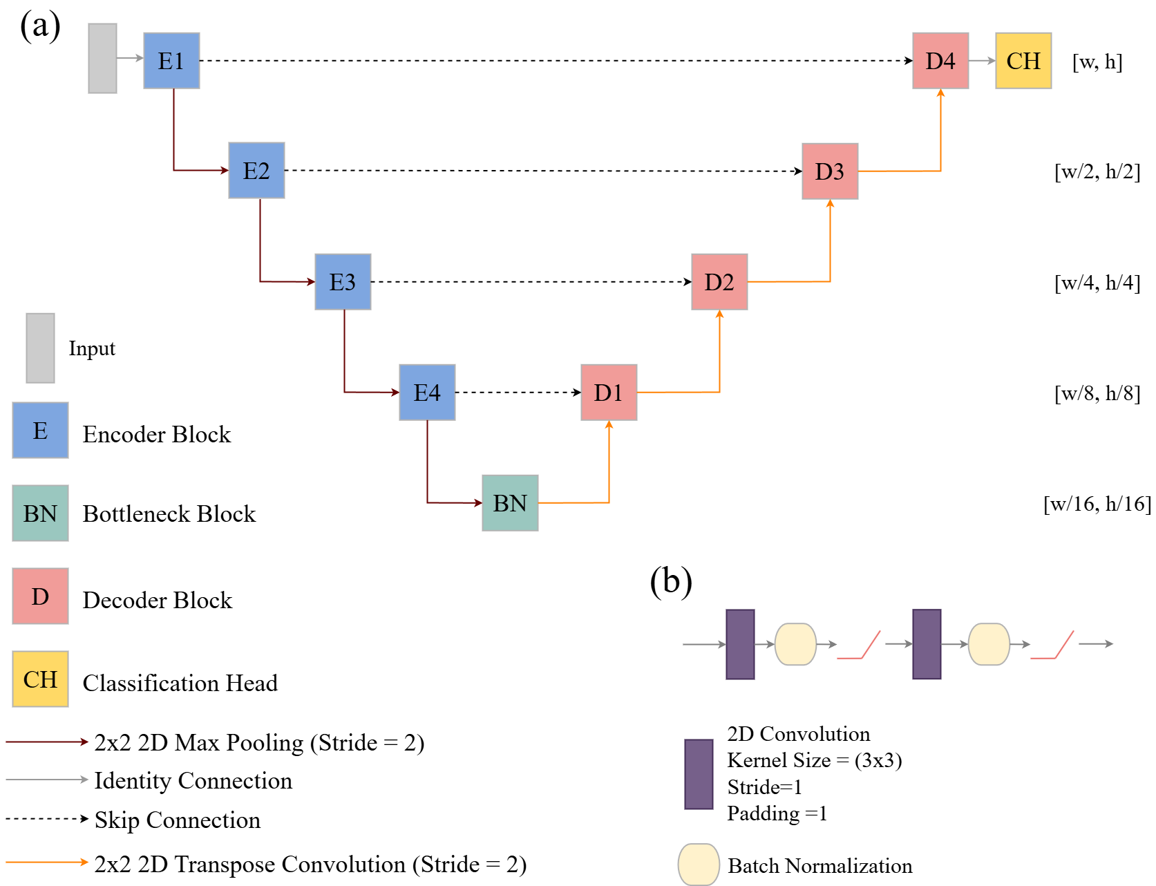
Another key characteristic of UNet and other semantic segmentation architectures is that there are no fully connected layers included. For our UNet implementation, the only required layers are 2D convolution, batch normalization, ReLU activation, and 2D transpose convolution. The final stage, termed the classification head, is designed to return logits for each predicted class at each pixel location using a 1x1 2D convolution layer. Essentially, the feature map values at each cell are processed to a set of class logits. A 1x1 kernel size means that there is no information shared between adjacent cells. As a result , 1x1 convolution on a cell-by-cell basis acts similarly to a fully connected layer where the output feature map values from the last decoder block serve as the input. The outputs are the class logits.
Now that we have discussed the basic architecture of UNet, we will build it using torch. Since we will only build the architecture and not train it, we do not need any data and only need to load the torch package. At the end of the chapter, we will build another UNet that uses a different encoder backbone.
14.3 Build Base UNet
14.3.1 Define Components
As the explanation above highlights, there are several repeating components in UNet. As a result, it would make sense to build out these separate components for re-use. Since architectures are built by subclassing nn_module(), we can build components that are then used within later subclasses. We specifically build three components:
- A double-convolution block to be used within the encoder, bottleneck, and encoder blocks
- A transpose convolution block for upsampling
- The classification head
The first code block below defines the double-convolution block, which we name doubleConvBlk(). It accepts the number of input channels or feature maps and the desired number of output feature maps. The data are then passed through the following sequence of operations:
2D 3x3 Convolution –> 2D Batch Normalization –> ReLU Activation –> 2D 3x3 Convolution –> 2D Batch Normalization –> ReLU Activation
The size of the input tensors in the spatial dimensions remain constant. Only the data abstractions and number of feature maps change. As with our examples from the prior chapters, the model architecture is defined within the initialize() method while how the data are passed through the architecture is defined by the forward() method.
doubleConvBlk <- torch::nn_module(
  initialize = function(inChn,
                        outChn){

    self$inChn <- inChn
    self$outChn <- outChn

    self$dConv <- torch::nn_sequential(
      torch::nn_conv2d(inChn,
                       outChn,
                       kernel_size=c(3,3),
                       stride=1,
                       padding=1),
      torch::nn_batch_norm2d(outChn),
      torch::nn_relu(inplace=TRUE),
      torch::nn_conv2d(outChn,
                       outChn,
                       kernel_size=c(3,3),
                       stride=1,
                       padding=1),
      torch::nn_batch_norm2d(outChn),
      torch::nn_relu(inplace=TRUE)
      )
  },

  forward = function(x){
    x <- self$dConv(x)
    return(x)
  }
)
2D transpose convolution with a kernel size of 2x2 and a stride of two is used to increase the spatial resolution of the feature maps within the encoder block. This is implemented by our upConvBlk() subclass, which is defined below. This consists of the following sequence of operations:
2D 2x2 Transpose Convolution –> 2D Batch Normalization –> ReLU Activation
In contrast to the double-convolution block, this architecture changes the spatial size or number of rows and columns of cells.
upConvBlk <- torch::nn_module(
  initialize = function(inChn,
                         outChn){

    self$inChn <- inChn
    self$outChn <- outChn

    self$upConv <- torch::nn_sequential(
      torch::nn_conv_transpose2d(inChn,
                                 outChn,
                                 kernel_size=c(2,2),
                                 stride=2),
      torch::nn_batch_norm2d(outChn),
      torch::nn_relu(inplace=TRUE)
    )
  },

  forward = function(x){
    x <- self$upConv(x)
    return(x)
  }
)
Our last component is the classification head, defined below as classiferBlk(). It consists of only a 2D 1x1 convolution operation. We use a stride of one so that each cell is processed. Since the kernel size is 1x1, there is no need for padding. The number of input channels or feature maps for this block is equal to the number of feature maps generated by the final decoder block while the number of output channels is equal to the number of classes being differentiated.
14.3.2 Define UNet
Now that we have our building blocks, we can use them to create the entire UNet architecture. This is defined below as unetMod() and by subclassing nn_module(). The subclasses defined above are used within the new subclass.
The architecture allows the user to define the number of input channels or predictor variables (inChn); number of classes being differentiated (nCls); and the number of feature maps produced by each encoder block (enChn), the bottleneck block (btnChn), and each decoder block (dcChn). Since there are four encoder and decoder blocks, the arguments for enchn and dcChn are vectors with a length of four.
Due to the use of skip connections, the data do not pass sequentially through the network. As a result, we cannot use nn_sequential() to build the entire network. Instead, we define each block separately. This includes all encoder blocks, the bottleneck, all decoder blocks, all upsampling operations in the decoder, and the classification head. It is important that the correct count of input channels/feature maps and output feature maps are defined for each block and using the user-defined inputs. If a layer in the architecture receives a different count of inputs than what is expected, it will fail. Depending on the type of error or the cause of the error, the model may fail either (1) when the subclass is created, (2) when an instance of the subclass is instantiated, or (3) when data are passed through the architecture.
There are a variety of means to build a UNet architecture with torch. We have tried to present a method that is straightforward. However, there are other means to define the architecture that would require less code.
How data pass through the architecture is defined by the forward() method. In order to merge outputs from the prior decoder block with those from the skip connection for a specific stage of the model, concatenation is performed along the channel dimension using torch_cat(). 2D max pooling is implemented with nnf_max_pool2d(). The forward() method returns the predicted class logits at each pixel location at the original spatial resolution of the input data with each channel holding logits for a specific class.
In torch there are both functional and class-based versions of some operations. For example, max pooling can be implemented with nnf_max_pool2d() or nn_max_poold2d(). Functional forms do not need to be instantiated prior to use and are prefixed with nnf_ as opposed to nn_.
unetMod <- torch::nn_module(
  "UNet",
  initialize  = function(inChn = 3,
                          nCls = 3,
                          enChn = c(16,32,64,128),
                          dcChn = c(128,64,32,16),
                          btnChn = 256){

    self$inChn = inChn
    self$nCls = nCls
    self$enChn = enChn
    self$dcChn = dcChn
    self$btnChn = btnChn

    self$e1 <- doubleConvBlk(inChn=inChn,
                             outChn=enChn[1])
    self$e2 <- doubleConvBlk(inChn=enChn[1],
                             outChn=enChn[2])
    self$e3 <- doubleConvBlk(inChn=enChn[2],
                             outChn=enChn[3])
    self$e4 <- doubleConvBlk(inChn=enChn[3],
                             outChn=enChn[4])

    self$dUp1 <- upConvBlk(inChn=btnChn,
                           outChn=btnChn)
    self$dUp2 <- upConvBlk(inChn=dcChn[1],
                           outChn=dcChn[1])
    self$dUp3 <- upConvBlk(inChn=dcChn[2],
                           outChn=dcChn[2])
    self$dUp4 <- upConvBlk(inChn=dcChn[3],
                           outChn=dcChn[3])

    self$d1 <- doubleConvBlk(inChn=btnChn+enChn[4],
                             outChn=dcChn[1])
    self$d2 <- doubleConvBlk(inChn=dcChn[1]+enChn[3],
                             outChn=dcChn[2])
    self$d3 <- doubleConvBlk(inChn=dcChn[2]+enChn[2],
                             outChn=dcChn[3])
    self$d4 <- doubleConvBlk(inChn=dcChn[3]+enChn[1],
                             outChn=dcChn[4])

    self$btn <- doubleConvBlk(inChn=enChn[4],
                         outChn=btnChn)

    self$ch <- classifierBlk(inChn=dcChn[4],
                             nCls=nCls)

  },

  forward = function(x){

    e1x <- self$e1(x)

    e1xMP <- torch::nnf_max_pool2d(e1x,
                                   kernel_size=c(2,2),
                                   stride=2,
                                   padding=0)

    e2x <- self$e2(e1xMP)

    e2xMP <- torch::nnf_max_pool2d(e2x,
                                   kernel_size=c(2,2),
                                   stride=2,
                                   padding=0)

    e3x <- self$e3(e2xMP)

    e3xMP <- torch::nnf_max_pool2d(e3x,
                                   kernel_size=c(2,2),
                                   stride=2,
                                   padding=0)

    e4x <- self$e4(e3xMP)

    e4xMP <- torch::nnf_max_pool2d(e4x,
                                   kernel_size=c(2,2),
                                   stride=2,
                                   padding=0)

    btnx <- self$btn(e4xMP)

    d1Upx <- self$dUp1(btnx)
    d1Cat <- torch::torch_cat(list(d1Upx, e4x), dim=2)
    d1x <- self$d1(d1Cat)

    d2Upx <- self$dUp2(d1x)
    d2Cat <- torch::torch_cat(list(d2Upx, e3x), dim=2)
    d2x <- self$d2(d2Cat)

    d3Upx <- self$dUp3(d2x)
    d3Cat <- torch::torch_cat(list(d3Upx, e2x), dim=2)
    d3x <- self$d3(d3Cat)

    d4Upx <- self$dUp4(d3x)
    d4Cat <- torch::torch_cat(list(d4Upx, e1x), dim=2)
    d4x <- self$d4(d4Cat)

    chx <- self$ch(d4x)

    return(chx)
  }
)
14.3.3 Explore Configuration
To test the model architecture, we will pass some random data through it. This requires first instantiating an instance of the model. The model instance below is designed to accept five channels or predictor variables and differentiate seven classes. Encoder blocks 1 through 4 will generated 16, 32, 64, and 128 feature maps, respectively, while the bottleneck block will produce 256 feature maps. Decoder blocks 1 through 4 will produce 128, 64, 32, and 16 feature maps, respectively. In UNet and UNet-like architectures, it is common to increase the number of feature maps produced through the encoder and decrease the number of feature maps produced through the decoder. The bottleneck generally has the largest number of output feature maps so that it can capture a variety of semantic information but at a reduced spatial resolution. Once an instance of the architecture is instantiated, we pass some randomized test data through it then print the result. Note that the model will fail if the data do not have the correct number of input predictor variables or channels. The example data have the following shape [mini-batch size, number of input channels, number of rows, number of columns]. So, our random test data mimic a mini-batch with 12 samples, 5 predictor variables or channels, and a size of 256x256 cells. The output has the same shape except that their are 7 output channels, each representing a logit for a specific class.
model <- unetMod(inChn=5,
                 nCls=7,
                 enChn=c(16,32,64,128),
                 dcChn=c(128,64,32,16),
                 btnChn=256)

predIn <- torch_rand(12,5,256,256)
predOut <- model(predIn)

predOut$shape
[1] 12 7 256 256Table 14.1 lists the number of trainable parameters in each layer of the UNet architecture as configured for five input channels and seven output classes. Each block in the encoder, bottleneck, and decoder consists of two 2D 3x3 convolution layers with associated batch normalization and ReLU activation. For a convolutional layer the number of trainable kernel weights is equal to the number of input feature maps times the number of output feature maps times the number of weights in each kernel (i.e., nine). Each kernel also as an associated bias term. For each batch normalization layer, the number of trainable parameters is equal to 2 times the number of input feature maps since there are scale and shift parameter for each input feature map. There are no trainable parameters associated with the max pooling or ReLU operations. For the 2x2 2D transpose convolution used for upsampling, the number of trainable parameters is equal to the number of input feature maps times the number out output feature maps times the number of weights in each kernel (i.e., four). As the table highlights, the majority of the trainable parameters are the kernel weights in the convolution and transpose convolution layers. The custom function, which was also used in the prior chapters, confirms the total number of trainable parameters in the architecture: 2,315,559.
| Layer | Kernel Weights | Kernel Biases | BN Scale | BN Shift |
|---|---|---|---|---|
| Encoder 1 | 3,024 | 32 | 32 | 32 |
| Max Pool 1 | 0 | 0 | 0 | 0 |
| Encoder 2 | 13,824 | 64 | 64 | 64 |
| Max Pool 2 | 0 | 0 | 0 | 0 |
| Encoder 3 | 55,296 | 128 | 128 | 128 |
| Max Pool 3 | 0 | 0 | 0 | 0 |
| Encoder 4 | 221,184 | 256 | 256 | 256 |
| Max Pool 4 | 0 | 0 | 0 | 0 |
| Bottleneck | 884,736 | 512 | 512 | 512 |
| Decoder Up 1 | 262,144 | 256 | 256 | 256 |
| Decoder 1 | 589,824 | 256 | 256 | 256 |
| Decoder Up 2 | 65,536 | 128 | 128 | 128 |
| Decoder 2 | 147,456 | 128 | 128 | 128 |
| Decoder Up 3 | 16,384 | 64 | 64 | 64 |
| Decoder 3 | 36,864 | 64 | 64 | 64 |
| Decoder Up 4 | 4,096 | 32 | 32 | 32 |
| Decoder 4 | 9,216 | 32 | 32 | 32 |
| Classification Head | 112 | 7 | 0 | 0 |
| Totals | 2,309,696 | 1,959 | 1,952 | 1,952 |
| Grand Total | 2,315,559 |
count_trainable_params <- function(model) {
  if (!inherits(model, "nn_module")) {
    stop("The input must be a torch nn_module.")
  }

  params <- model$parameters

  trainable_params <- lapply(params, function(param) {
    if (param$requires_grad) {
      as.numeric(prod(param$size()))
    } else {
      0
    }
  })

  total_trainable_params <- sum(unlist(trainable_params))

  return(total_trainable_params)
}count_trainable_params(model)[1] 2315559We will not train the UNet in this chapter. We explore training, validation, and using semantic segmentation models in the next two chapters using geodl and luz. Our goal in this chapter is to introduce how a semantic segmentation architecture can be built using torch.
14.4 MobileNetv2 UNet
Since the encoder component of a UNet or similar semantic segmentation architecture serves the same purpose as the CNN component of a scene classification architecture, it is possible to replace the encoder with a pre-defined CNN architecture such as one from the ResNet, InceptionNet, VGGNet, DenseNet, or MobileNet families. Since many of these architectures have been pre-trained using large datasets, such as ImageNet, this allows for instantiating the model using pre-trained weights for the encoder component only while initializing the decoder using random weights. The encoder can be frozen during training or updated but from the non-random initial state. This is one means to implement transfer learning and may allow for obtaining accurate results with a small training set.
In the example below, we have built a UNet architecture that uses the convolutional component of the MobileNetv2 model. This was modified from a Posit blog post by Sigrid Keydana. The architecture is conceptualized in Figure 14.2. Since we need to extract intermediate feature maps for use along the skip connections, it is not possible to pass the input data through the MobileNetv2 architecture to obtain the final output. Instead, the architecture must be split up so that the intermediate outputs can be used along the skip connections. It can be tricky to determine how to split the architecture. The goal is to split the architecture when the spatial dimensions of the array decrease in size in order to match the appropriate stage of the UNet encoder and associated decoder. This generally requires some exploration of the model architecture and how it has been built or coded.
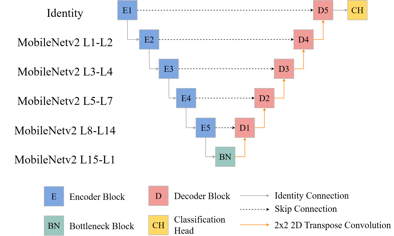
Some other key components of the architecture include the requirements to use three input channels so that ImageNet weights can be implemented, the use of five encoder and five decoder blocks, the ability to load pre-trained ImageNet weights for the encoder, and the ability to freeze the encoder and only train the decoder. The number of output channels for each encoder block are also fixed since these are defined internally by the MobileNetv2 architecture. However, the user can specify the number of feature maps to generate for each decoder block.
mobileUnetMod <- torch::nn_module(
  "MobileUNet",
  initialize  = function(nCls = 3,
                         dcChn = c(256,128,64,32,16),
                         pretrainedEncoder = TRUE,
                         freezeEncoder = TRUE){

    self$nCls = nCls
    self$dcChn = dcChn
    self$pretrainedEncoder = pretrainedEncoder
    self$freezeEncoder = freezeEncoder

    self$base_model <- torchvision::model_mobilenet_v2(pretrained = pretrainedEncoder)

    self$stages <- torch::nn_module_list(list(
      torch::nn_identity(),
      self$base_model$features[1:2],
      self$base_model$features[3:4],
      self$base_model$features[5:7],
      self$base_model$features[8:14],
      self$base_model$features[15:18]
    ))

    self$e1 <- torch::nn_sequential(self$stages[[1]])

    self$e2 <- torch::nn_sequential(self$stages[[2]])

    self$e3 <- torch::nn_sequential(self$stages[[3]])

    self$e4 <- torch::nn_sequential(self$stages[[4]])

    self$e5 <-  torch::nn_sequential(self$stages[[5]])

    self$btn <- torch::nn_sequential(self$stages[[6]])

    if(freezeEncoder == TRUE){
      for (par in self$parameters) {
        par$requires_grad_(FALSE)
      }
    }

    self$dUp1 <- upConvBlk(inChn=320,
                           outChn=320)
    self$dUp2 <- upConvBlk(inChn=dcChn[1],
                           outChn=dcChn[1])
    self$dUp3 <- upConvBlk(inChn=dcChn[2],
                           outChn=dcChn[2])
    self$dUp4 <- upConvBlk(inChn=dcChn[3],
                           outChn=dcChn[3])
    self$dUp5 <- upConvBlk(inChn=dcChn[4],
                           outChn=dcChn[4])

    self$d1 <- doubleConvBlk(inChn=320+96,
                             outChn=dcChn[1])
    self$d2 <- doubleConvBlk(inChn=dcChn[1]+32,
                             outChn=dcChn[2])
    self$d3 <- doubleConvBlk(inChn=dcChn[2]+24,
                             outChn=dcChn[3])
    self$d4 <- doubleConvBlk(inChn=dcChn[3]+16,
                             outChn=dcChn[4])
    self$d5 <- doubleConvBlk(inChn=dcChn[4]+3,
                             outChn=dcChn[5])

  self$ch <- classifierBlk(inChn=dcChn[5],
                           nCls=nCls)

  },

  forward = function(x){

    e1x <- self$e1(x)
    e2x <- self$e2(e1x)
    e3x <- self$e3(e2x)
    e4x <- self$e4(e3x)
    e5x <- self$e5(e4x)
    btnx <- self$btn(e5x)

    d1Upx <- self$dUp1(btnx)
    d1Cat <- torch::torch_cat(list(d1Upx, e5x), dim=2)
    d1x <- self$d1(d1Cat)

    d2Upx <- self$dUp2(d1x)
    d2Cat <- torch::torch_cat(list(d2Upx, e4x), dim=2)
    d2x <- self$d2(d2Cat)

    d3Upx <- self$dUp3(d2x)
    d3Cat <- torch::torch_cat(list(d3Upx, e3x), dim=2)
    d3x <- self$d3(d3Cat)

    d4Upx <- self$dUp4(d3x)
    d4Cat <- torch::torch_cat(list(d4Upx, e2x), dim=2)
    d4x <- self$d4(d4Cat)

    d5Upx <- self$dUp5(d4x)
    d5Cat <- torch::torch_cat(list(d5Upx, e1x), dim=2)
    d5x <- self$d5(d5Cat)

    c4x <- self$ch(d5x)

    return(c4x)
  }
)
To test the new model architecture, we first instantiate an instance of the subclass then use it to predict random data. The output shape is as expected. Using our parameter counting function, we can see that the number of trainable parameters when the encoder is frozen is 2,954,791. When the encoder is unfrozen, or trainable, the number of trainable parameters is 6,459,663. This confirms that the configuration is actually freezing components of the model as desired.
model <- mobileUnetMod(nCls=7,
                       pretrainedEncoder=TRUE,
                       freezeEncoder=TRUE)

predIn <- torch_rand(12,3,256,256)
predOut <- model(predIn)

predOut$shape
[1] 12 7 256 256model <- mobileUnetMod(nCls=7,
pretrainedEncoder=TRUE,
freezeEncoder=TRUE)
count_trainable_params(model)[1] 2954791model <- mobileUnetMod(nCls=7,
pretrainedEncoder=TRUE,
freezeEncoder=FALSE)
count_trainable_params(model)[1] 645966314.5 Concluding Remarks
Now that you know how to build a UNet architecture, we will move on to implementing geospatial semantic segmentation using the geodl package.
14.6 Questions
- Explain the purpose of skip connections in the UNet architecture.
- How is 2D transpose convolution for upsampling different from interpolation methods, such as bilinear interpolation?
- A convolutional layer uses a 3x3 kernel, accepts 10 input feature maps, and generates 20 output feature maps. How many trainable kernel weights and biases are associated with the layer?
- How many trainable parameters would be associated with a batch normalization layer applied to the output of the convolutional layer from Question 3?
- Explain how 1x1 2D convolution can be used to perform pixel-by-pixel classification.
- When using a kernel size of 3x3 and a stride of 1, why is it necessary to add a padding of 1 to not decrease the size of image arrays or feature maps in the spatial dimensions?
- An input image has spatial dimensions of 160x160 cells. What would be the size of the array in the spatial dimensions after the bottleneck layer if the encoder includes 4 blocks?
- A UNet architecture is able to make predictions on different size images than those used to train it. This is generally not the case for a CNN architecture for scene classification tasks. Explain why this is the case.
14.7 Exercises
The UNet-ID architecture augments UNet to support instance segmentation as opposed to semantic segmentation. The goal of this exercise is to build this architecture from scratch by subclassing nn_module(). The architecture was introduced in the following paper, which has been included in the exercise folder for the chapter as a PDF (remotesensing-12-01544-v2.pdf). The paper is available in open access here.
Wagner, F.H., Dalagnol, R., Tarabalka, Y., Segantine, T.Y., Thomé, R. and Hirye, M.C., 2020. U-net-id, an instance segmentation model for building extraction from satellite images—case study in the joanópolis city, brazil. Remote Sensing, 12(10), p.1544.
Background Questions
- What is the difference between semantic and instance segmentation?
- Write a paragraph explaining the components of the traditional UNet architecture. Please discuss the architecture in detail. Someone should be able to use your description to build the architecture by subclassing
nn_module(). - Using the paper cited above, explain how UNet-ID augments the UNet architecture for instance segmentation. Please discuss the architecture in detail. Someone should be able to use your description to build the architecture by subclassing
nn_module(). - Explain the input data requirements for UNet-ID and how the requirements are different than UNet.
Task
Build the UNet-ID architecture from scratch by subclassing nn_module(). Test the architecture by instantiating it and predicting some randomly generated data of the correct shape.
Hints and Suggestions
- Try drawing out the architecture on paper before building it out in code.
- It is easiest to build the architecture up in pieces. You should not build the entire architecture in a single
nn_module()subclass. - Make sure to reuse components when possible.
- Figures 1 and 2 in the paper and the associated text should be your primary source material.
- The model should generate three output predictions.
- The input data are cropped before being passed to the architecture, and the final feature maps are cropped further. You do not need to code these components relating to resizing the tensors. In other words, you can skip the resizing steps.