| Geometry Type | Description |
|---|---|
| POINT | Each point treated as a single record |
| MULTIPOINT | Allows multiple points to be treated like a single record |
| LINESTRING | Series of coordinates connected as a line |
| MULTILINESTRING | Allows for multiple lines to be treated as one record |
| POLYGON | Series of coordinates forming a closed, areal shape |
| MULTIPOLYGON | Allows multiple polygons to be treated as a single record |
| GEOMETRYCOLLECTION | Objects where rows/records can have different geometries |
24 Vector Geoprocessing (sf)
24.1 Topics Covered
- Read and write geospatial vector data with sf
- Apply general data wrangling and summarization to vector geospatial data using dplyr
- Work with coordinate reference systems and bounding boxes
- Convert between geometry types and generate bounding geometries
- Perform proximity analysis/buffering
- Perform geoprocessing and vector overlay
- Summarize point and line features relative to polygons
- Geometry simplification, spatial sampling, and tessellation
24.2 Introduction
24.2.1 Overview of sf
In this chapter we explore a wide variety of techniques for working with and analyzing vector geospatial data in R. Specifically, we focus on methods made available in the sf package. If you have worked with PostgreSQL and PostGIS, you will observe lots of similarities. For example, functions designed to operate on spatial data in sf and PostGIS are both commonly prefixed with “st_”. Also, they both make use of an object-based vector data model where the geometry and attributes are stored in the same table. In other words, the geometric data are simply stored as another column in the table alongside feature attributes. One benefit of this structure is that we can perform the same data preprocessing, manipulation, wrangling, and querying techniques on sf object that we have already used for data frames/tibbles, such as the methods made available by dplyr.
sf offers several geometry types as summarized in Table 24.1. Other than POINT, LINESTRING, and POLYGON features, it is possible to create MULTIPOINT, MULTILINESTRING, and MULTIPOLYGON features where multiple, and potentially noncontiguous, geographic features are treated as one record in the table. Further, it is not required that all records or features in the object have the same geometry type. This is the purpose of the GEOMETRYCOLLECTION data type. The st_cast() function is used to convert between geometry types. Geometric errors can be detected using st_is_valid() while st_make_valid() allows for correcting geometric errors. Note that corrections may not always be successful (only certain types of geometric errors can be detected and corrected).
sf also provides spatial logical test that return TRUE or FALSE, which can be useful for conducting spatial queries. These tests are described in Table 24.2.
| Function | Use |
|---|---|
| st_intersects() | Do A and B intersect? |
| st_disjoint() | Are A and B disjoint? |
| st_touches() | Do A and B touch? |
| st_crosses() | Do A and B cross? |
| st_within() | Is A within B? |
| st_contains() | Does A contain B? |
| st_overlaps() | Do A and B overlap? |
| st_equals() | Are A and B identical? |
| st_covers() | Does A cover B? |
| st_covered_by() | Is A covered by B? |
| st_is_within_a_distance() | Is A within a given distance of B? |
Methods are also available for obtaining or transforming the datum/projection information for a layer. For example, st_crs() provides the datum/projection information while st_tranform() allows for converting between datums/projections. This can be useful when layers being used in an analysis do not have the same projection or coordinate reference system.
When performing overlay or spatial analysis involving multiple data layers using sf, the layers should use the same datum/projection information. If they do not, you can use st_transform() for datum/projection conversion.
There are also functions available for calculating geometric properties as described in Table 24.3. These calculations are made relative to the object’s datum/projection or a specified coordinate reference system.
It is generally best to calculate geometric properties using a projected coordinate system as opposed to a geographic coordinate system (i.e., latitude and longitude).
| Function | Use |
|---|---|
| st_area() | Calculate area of polygon relative to a datum/projection |
| st_length() | Calculate length of a line relative to a datum/projection |
| st_perimeter() | Calculate perimeter of a polygon relative to a datum/projection |
| st_distance() | Calculate distance between two geometries |
24.2.2 Read Data
We first load in the required packages including the tidyverse, sf, and tmap. Loading the tidyverse also loads dplyr, which is used extensively in this chapter. We use a variety of data layers, and all of the vector layers are stored in the chpt24.gpkg geopackage.
- circle: a circle
- triangles: a triangle
- extent: bounding box extent of circle and triangle
- interstates: interstates in West Virginia as lines
- rivers: major rivers in West Virginia as lines
- towns: point features of large towns in West Virginia
- wv_counties: West Virginia county boundaries as polygons
- harvest.csv: CSV table of deer harvest data by county from the West Virginia Division of Natural Resources (WVDNR)
- tornadoesUS: point features of tornadoes across US
- citiesUS: point features of cities in the US
- interstatesUS: interstates in US as lines
- Us_eco_ref_l3US: ecological regions of the US as polygons
- statesUS: US state boundaries
All vector files are read in using the st_read() function from sf. This generates an sf object, which functions similar to a data frame/tibble other than that the geometry data are also included in the table in a column named “geometry”. Tabulated data as a CSV file, harvest.csv, are loaded using read_csv() from readr.
When reading a file from a database, such as a ESRI File Geodatabase or a GeoPackage, the dsn argument provides the name of the database. This is the first argument for st_read(), which is followed by the name of the layer that is being read from the database. If the file is not within a database, such as a shapefile or GeoJSON file, you do not need to provide an argument for the dsn parameter. Setting the quiet parameter to TRUE minimizes the amount of information printed.
Printing the first set of rows from the rivers layer, we can see that the data are formatted as a table where each row represents a spatial feature and the “geometry” column stores the geometric data. All other columns are attributes associated with the spatial object.
fldPth <- "gslrData/chpt24/data/"

circle <- st_read(dsn=str_glue("{fldPth}chpt24.gpkg"),
                  "circle",
                  quiet=TRUE)

triangle <- st_read(dsn=str_glue("{fldPth}chpt24.gpkg"),
                    "triangle",
                    quiet=TRUE)

ext <- st_read(dsn=str_glue("{fldPth}chpt24.gpkg"),
               "extent",
               quiet=TRUE)

inter <- st_read(dsn=str_glue("{fldPth}chpt24.gpkg"),
                 "interstates",
                 quiet=TRUE)

rivers <- st_read(dsn=str_glue("{fldPth}chpt24.gpkg"),
                  "rivers",
                  quiet=TRUE)

towns <- st_read(dsn=str_glue("{fldPth}chpt24.gpkg"),
                 "towns",
                 quiet=TRUE)

wv_counties <- st_read(dsn=str_glue("{fldPth}chpt24.gpkg"),
                 "wv_counties",
                 quiet=TRUE)

harvest <- read_csv(str_glue("{fldPth}harvest.csv")) |>
  mutate_if(is.character, as.factor)

torn <- st_read(dsn=str_glue("{fldPth}chpt24.gpkg"),
                "tornadoesUS",
                quiet=TRUE)

us_cities <- st_read(dsn=str_glue("{fldPth}chpt24.gpkg"),
                     "citiesUS",
                     quiet=TRUE)

us_inter <- st_read(dsn=str_glue("{fldPth}chpt24.gpkg"),
                     "interstatesUS",
                     quiet=TRUE)

eco <- st_read(dsn=str_glue("{fldPth}chpt24.gpkg"),
               "us_eco_ref_l3US",
               quiet=TRUE)

states <- st_read(dsn=str_glue("{fldPth}chpt24.gpkg"),
                  "statesUS",
                  quiet=TRUE)
24.3 Data Wrangling and Query with dplyr
Let’s start by mapping the ecological region boundaries using tmap. We are using the fill color to show the Level 1 ecoregion name as a qualitative/categorical variable. We are also plotting the legend outside of the map space.
tm_shape(eco)+
  tm_polygons(fill="NA_L1NAME")+
  tm_layout(legend.outside=TRUE)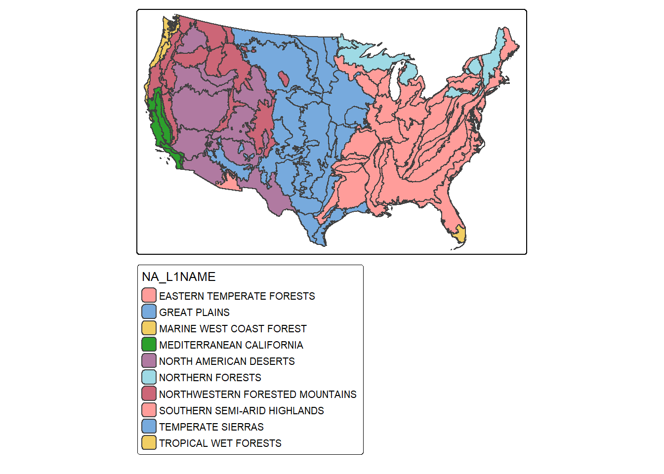
Since sf objects act as data frames, we can work with and manipulate them using a variety of functions that accept data frames. In the next code block we use dplyr to count the number of polygons belonging to each Level 1 ecoregion. The result is a tibble. We can confirm that the eastern temperate forest has the largest number of polygons associated with it. This process is the same as working with any data frame/tibble, which is one of the benefits of using sf to read vector data into R. In order to remove the geometric information from the data layer, we use the st_drop_geometry() function from sf. We use this throughout the chapter when we do not need the geometry information included in the output.
eco_l1_names <- eco |>
  group_by(NA_L1NAME) |>
  count() |>
  st_drop_geometry()

eco_l1_names |> gt()| NA_L1NAME | n |
|---|---|
| EASTERN TEMPERATE FORESTS | 890 |
| GREAT PLAINS | 46 |
| MARINE WEST COAST FOREST | 75 |
| MEDITERRANEAN CALIFORNIA | 40 |
| NORTH AMERICAN DESERTS | 13 |
| NORTHERN FORESTS | 43 |
| NORTHWESTERN FORESTED MOUNTAINS | 38 |
| SOUTHERN SEMI-ARID HIGHLANDS | 2 |
| TEMPERATE SIERRAS | 11 |
| TROPICAL WET FORESTS | 92 |
Records, rows, or geospatial features can be extracted using the filter() function from dplyr. In the next code block, we extract out all features that are within the Great Plains Level 1 ecoregion. We then map the extracted features and use the fill color to differentiate the Level 2 ecoregions. Note that we use droplevels() here to remove any Level 2 names that are not in the extracted subset of Level 1 ecoregions. This is common practice when subsetting factors, as you may recall.
eco_gp <- eco |>
  filter(NA_L1NAME=="GREAT PLAINS")

eco_gp$NA_L2NAME <- eco_gp$NA_L2NAME |>
  as.factor() |> droplevels()

tm_shape(eco_gp)+
  tm_polygons(fill="NA_L2NAME")+
  tm_layout(legend.outside=TRUE)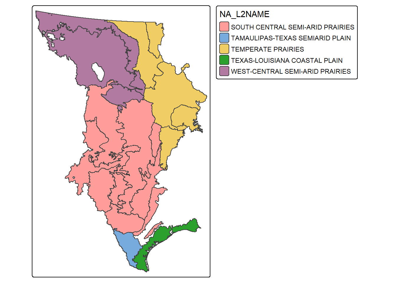
Again, since sf objects behave as data frames/tibbles, we can explore the tabulated data using a variety of tidyverse functions and methods. As an example, we use ggplot2 to compare county-level population by sub-region of the US. Since the geographic information is not needed here, it is simply ignored.
ggplot(states, aes(x=SUB_REGION,
                   y=POP2000,
                   fill=SUB_REGION))+
  geom_boxplot()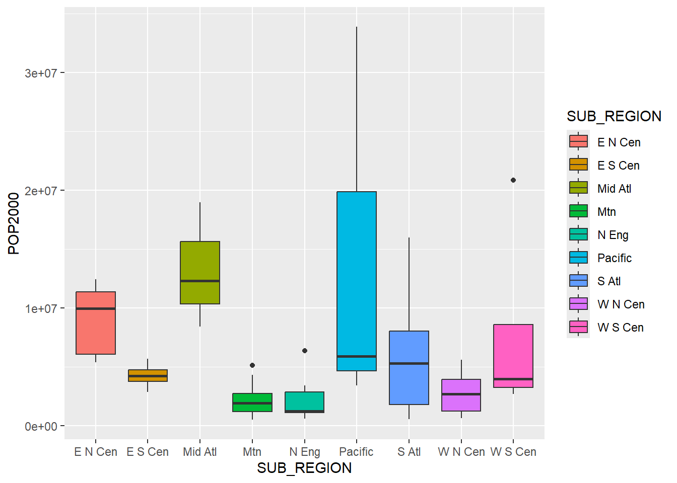
As a similar example, we now use dplyr to obtain the mean county population for each sub-region. The geometry data are automatically included in the output even if the geometry column is not selected or used. As demonstrated above, the geometry information can be removed if not needed using st_drop_geometry().
states |>
  group_by(SUB_REGION) |>
  summarize(mn_pop = mean(POP2000)) |>
  st_drop_geometry() |>
gt()| SUB_REGION | mn_pop |
|---|---|
| E N Cen | 9031007 |
| E S Cen | 4255703 |
| Mid Atl | 13223954 |
| Mtn | 2271537 |
| N Eng | 2320420 |
| Pacific | 14395723 |
| S Atl | 5752129 |
| W N Cen | 2748248 |
| W S Cen | 7861213 |
Each tornado point has a Fujita scale attribute, a measure of tornado intensity. We now count the number of tornadoes by Fujita category. As expected, severe tornadoes occur much less frequently. We next extract all tornadoes that have a Fujita value greater than or equal to 3 using dplyr and plot them as points using tmap.
torn |>
  group_by(F_SCALE) |>
  count() |>
  st_drop_geometry() |>
gt()| F_SCALE | n |
|---|---|
| 0 | 1236 |
| 1 | 531 |
| 2 | 168 |
| 3 | 58 |
| 4 | 6 |
| 5 | 1 |
torn_hf <- torn |>
  filter(F_SCALE >= 3)

tm_shape(states)+
  tm_polygons(fill="tan")+
  tm_shape(torn_hf)+
  tm_bubbles(fill="red")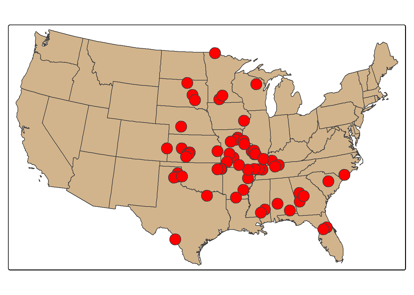
It is also possible to subset columns or attributes using the select() function from dplyr. Using this function, we extract out only the state name, sub-region, and population attributes using the code below. Note again that the geometric information is automatically included even though it was not selected.
Rows: 49
Columns: 4
$ STATE_NAME <chr> "Washington", "Montana", "Maine", "North Dakota", "South Da…
$ SUB_REGION <chr> "Pacific", "Mtn", "N Eng", "W N Cen", "W N Cen", "Mtn", "E …
$ POP2000    <int> 5894121, 902195, 1274923, 642200, 754844, 493782, 5363675, …
$ Shape      <MULTIPOLYGON [m]> MULTIPOLYGON (((-1954354 14..., MULTIPOLYGON (…
24.4 Table Joins
Tabulated data can be joined to spatial features if they share a common field or attribute. This is known as a table join. The goal of the next code block is to join the deer harvest tabulated data to the county boundaries. First, we change the second column’s name in the deer harvest table to “NAME” as opposed to “COUNTY” using rename() from dplyr so that the column name matches that of the polygon features. We then use left_join() from dplyr to associate the data using the common “NAME” field. Lastly, we map the total number of deer harvested by county using tmap.
harvest <- harvest |>
  rename("NAME" = "COUNTY")

counties_harvest <- inner_join(wv_counties,
                               harvest, by="NAME")

tm_shape(counties_harvest) +
  tm_polygons(fill="TOTALDEER",
              fill.legend = tm_legend(title="Harvest"),
              fill.scale= tm_scale_continuous(values="brewer.reds"))+
  tm_compass()+
  tm_scalebar()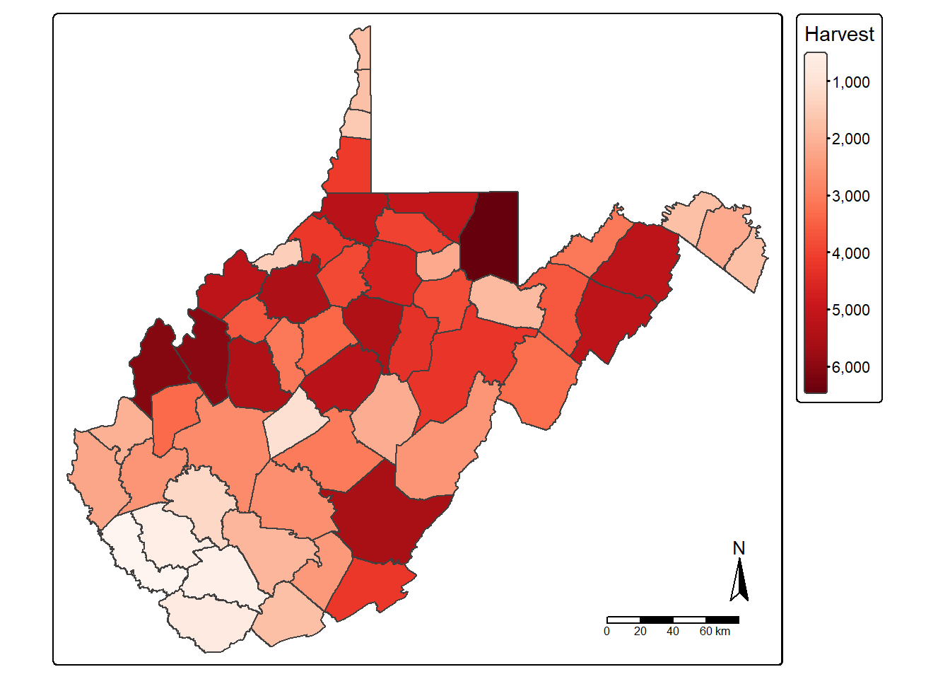
New attribute columns can be generated using the mutate() function from dplyr. Using this function, we calculate the density of deer harvested as deer per square mile using the “TOTALDEER” and “SQUARE_MIL” fields. The density is written to a new column called “DEN”, and the result is mapped. Next, we use the filter() function to extract out and map all counties that have a deer harvest density greater than five deer per square mile.
counties_harvest <- counties_harvest |>
  mutate(DEN = TOTALDEER/SQUARE_MIL
)


tm_shape(counties_harvest)+
    tm_polygons(fill="DEN",
              fill.legend = tm_legend(title="Harvest Density"),
              fill.scale= tm_scale_continuous(values="brewer.reds"))+
  tm_compass()+
  tm_scalebar()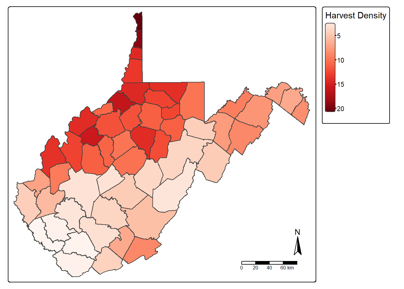
counties_harvest_sub <- counties_harvest |>
  filter(DEN > 5)

tm_shape(counties_harvest)+
  tm_polygons(fill="gray")+
  tm_shape(counties_harvest_sub)+
  tm_polygons(fill="DEN",
              fill.legend = tm_legend(title="Harvest Density"),
              fill.scale= tm_scale_continuous(values="brewer.reds"))+
  tm_compass()+
  tm_scalebar()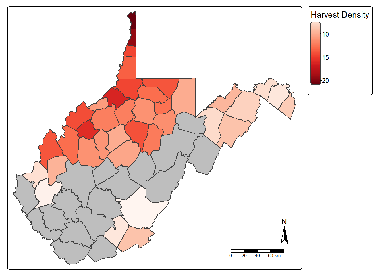
The st_area() function is used to calculate area for polygon features. The area is returned in the map units unless another datum/projection is specified. In our example, the units are square meters since the data are projected to a UTM coordinate system. In the following code block, we calculate area in hectares and write the values to a new column called “hec” then calculate density again using hectares as opposed to square meters.
counties_harvest$hec <- counties_harvest |>
  st_area()*0.0001
counties_harvest <- counties_harvest |>
  mutate(DEN2 = TOTALDEER/hec)

tm_shape(counties_harvest)+
  tm_polygons(fill="DEN2",
              fill.legend = tm_legend(title="Harvest Density"),
              fill.scale= tm_scale_continuous(values="brewer.reds"))+
  tm_compass()+
  tm_scalebar()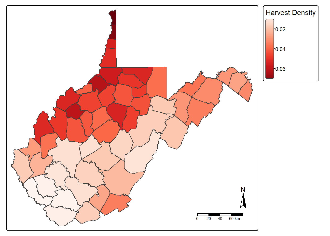
24.5 Geometry Type Conversions
24.5.1 Bounding Boxes and Centroids
The st_bbox() function is used to extract the bounding box coordinates for a layer. It does not create a spatial feature. To convert the bounding box coordinates to a spatial feature, we use the st_make_grid() function to create a grid that covers the extent of the bounding box with a single grid cell. This is a bit of a trick, but it works well. In the map, the bounding box for West Virginia is shown in red.
bb_wv <- wv_counties |>
  st_bbox() |>
  st_make_grid(n=1)

tm_shape(bb_wv)+
  tm_borders(col="red", lwd=2)+
  tm_shape(wv_counties)+
  tm_polygons(fill="tan")
st_centroid() is used to extract the centroid coordinates of each polygon feature and returns a POINT geometry. The centroid does not always occur inside of the polygon that it is the center of (for example, a “C-shaped” island or a doughnut). st_point_on_surface() provides an alternative in which a point within the polygon is returned. When points are generated from polygons, all the attributes are also copied, as demonstrated by printing the column names.
wv_centroids <- wv_counties |>
  st_centroid()

tm_shape(wv_counties)+
  tm_polygons(fill="tan")+
  tm_shape(wv_centroids)+
  tm_bubbles(fill="red", size=1)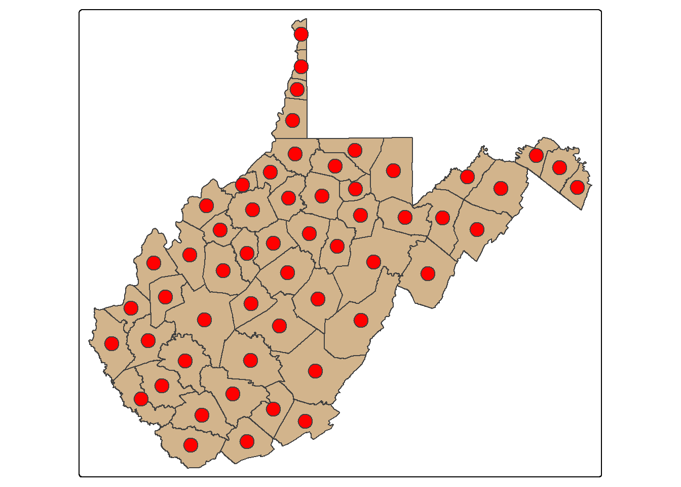
names(wv_centroids) [1] "AREA" "PERIMETER" "NAME" "STATE" "FIPS"
[6] "STATE_ABBR" "SQUARE_MIL" "POP2000" "POP00SQMIL" "MALE2000"
[11] "FEMALE2000" "MAL2FEM" "UNDER18" "AIAN" "ASIA"
[16] "BLACK" "NHPI" "WHITE" "AIAN_MORE" "ASIA_MORE"
[21] "BLK_MORE" "NHPI_MORE" "WHT_MORE" "HISP_LAT" "F1900"
[26] "F1910" "F1920" "F1930" "F1940" "F1950"
[31] "F1960" "F1970" "F1980" "F1991" "F1992"
[36] "F1993" "F1994" "F1995" "F1996" "F1997"
[41] "F1998" "F1999" "F1990" "F2000" "F2001"
[46] "F2002" "F2003" "F2004" "F2005" "F2006"
[51] "Shape" 24.5.2 Thiessen/Voronoi Polygons
Thiessen or Voronoi polygons represent the areas that are closer to one point feature than any other feature in a dataset. st_voronoi() can generate these polygons; however, this only works when points are aggregated to MULTIPOINT features, so we use the st_union() function to make this conversion. The result is a GEOMETRYCOLLECTION, which is converted back to a POINT geometry using st_cast(). We then extract out the polygon extents within the state extent using st_intersection(). We explain these additional functions later in this chapter. In short, this process serves as a means to convert points to polygons.
vor_poly <- wv_centroids |>
  st_union() |>
  st_voronoi() |>
  st_cast()

wv_diss <- wv_counties |>
  group_by(STATE) |>
  summarize(totpop = sum(POP2000))

vor_poly2 <- st_intersection(vor_poly, wv_diss)

tm_shape(wv_diss)+
  tm_polygons(col="tan")+
  tm_shape(vor_poly2)+
  tm_borders(col="red", lwd=2)+
  tm_shape(wv_centroids)+
  tm_bubbles(col="blue")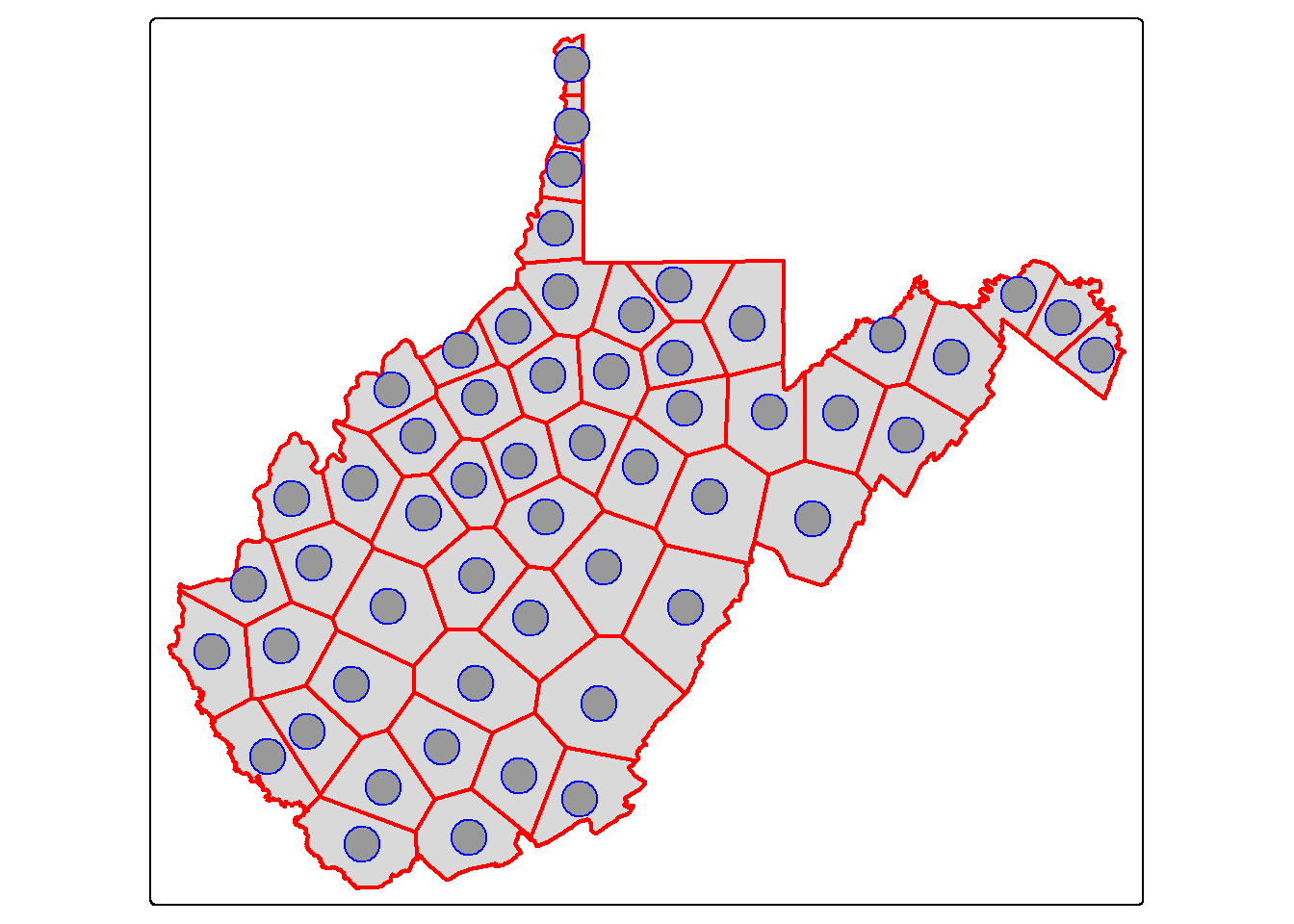
24.5.3 Convex Hull
A convex hull is a bounding geometry that encompasses features without any concave angles. Think of this as stretching a rubber band around the margin points in a dataset. A convex hull can be generated using the st_convex_hull() function. Similar to st_voronoi(), POINT geometries must first be converted to MULTIPOINT. It is also possible to generate a concave hull using st_concave_hull(). The degree of concavity is specified using a concavity parameter.
ch <- wv_centroids |>
  st_union() |>
  st_convex_hull()

tm_shape(wv_counties)+
  tm_polygons(col="tan")+
  tm_shape(wv_centroids)+
  tm_bubbles(col="red", size=1)+
  tm_shape(ch)+
  tm_borders(col="blue", lwd=2)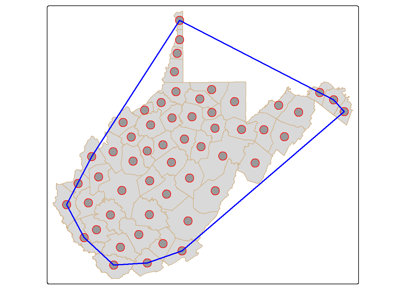
24.6 Spatial Joins
In contrast to a table join, a spatial join associates features based on spatial co-occurrence as opposed to a shared or common attribute. We use st_join() to spatially join the cities and states. The result is a POINT geometry with each city containing its original attributes plus the attributes for the state in which it occurs. To demonstrate this, we symbolize the points using the “SUB_REGION” field, which was initially attributed to the states layer.
cities2 <- st_join(us_cities, states)

tm_shape(states)+
  tm_polygons(fill="tan")+
  tm_shape(cities2)+
  tm_bubbles(fill="SUB_REGION", size=.6)+
  tm_layout(legend.outside = TRUE)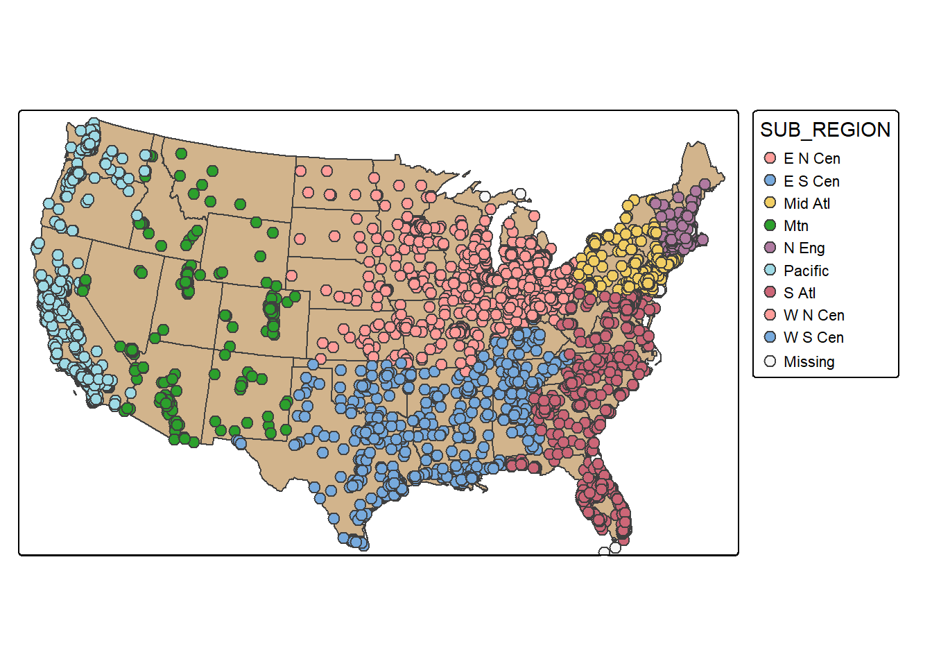
24.7 Random Sampling using the Table
Randomly sampling spatial features using dplyr is the same as randomly sampling records or rows from any data frame or tibble. In the first example, we demonstrate simple random sampling without replacement. The replace argument is set to FALSE to indicate that we do not want features to be selected multiple times. The result is 100 randomly selected cities. Since this is random, we will obtain a different result each time we run the code unless we set the random seed (set.seed()). It is also possible to stratify the sampling using group_by(). In the second example, we select 10 random cities per sub-region. To confirm that the desired result was obtained, we next create a table that provides a count of selected cities by sub-region.
cities_rswor <- cities2 |>
  sample_n(100, replace=FALSE)

tm_shape(states)+
  tm_polygons(fill="tan")+
  tm_shape(cities2)+
  tm_bubbles(fill="black", size=.5)+
  tm_shape(cities_rswor)+
  tm_bubbles(fill="red")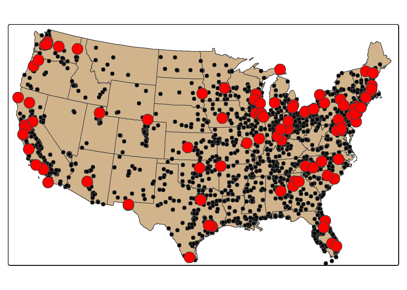
set.seed(42)
cities_srswor <- cities2 |>
  group_by(SUB_REGION) |>
  sample_n(10, replace=FALSE)

cities_srswor |>
  group_by(SUB_REGION) |>
  count() |>
  st_drop_geometry()
# A tibble: 10 × 2
SUB_REGION n
* <chr> <int>
1 E N Cen 10
2 E S Cen 10
3 Mid Atl 10
4 Mtn 10
5 N Eng 10
6 Pacific 10
7 S Atl 10
8 W N Cen 10
9 W S Cen 10
10 <NA> 10tm_shape(states)+
tm_polygons(fill="tan")+
tm_shape(cities_srswor)+
tm_bubbles(fill="SUB_REGION", size=.6)+
tm_layout(legend.outside = TRUE)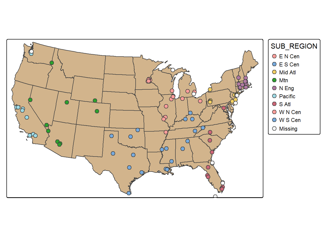
24.8 Geoprocessing
24.8.1 Boundary Generalization (Dissolve)
Dissolve is used for boundary generalization. For example, you can dissolve county boundaries to state boundaries or state boundaries to the country boundary. In the example, we obtain sub-region boundaries from the state boundaries. If you would like to include a summary of some attributes relative to the dissolved features, you can include a summary() function from dplyr. Below, we sum the population of all the states in each sub-region and write the result to a column called “totpop”. In the second example, we generate the West Virginia state boundary from the county boundaries. Since all counties have the same value in the “STATE” field, a single feature is returned. We have also summed the population for each county, which results in the total state population.
sub_regions <- states |>
  group_by(SUB_REGION) |>
  summarize(totpop = sum(POP2000))

tm_shape(sub_regions)+
  tm_polygons(fill="SUB_REGION")+
  tm_layout(legend.outside = TRUE)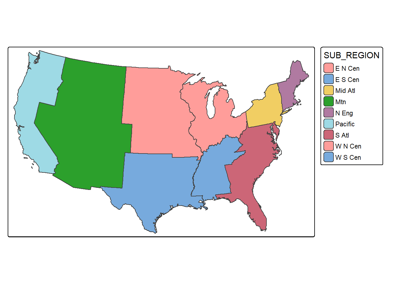
wv_diss <- wv_counties |>
  group_by(STATE) |>
  summarize(totpop = sum(POP2000))

tm_shape(wv_diss)+
  tm_polygons(fill="tan")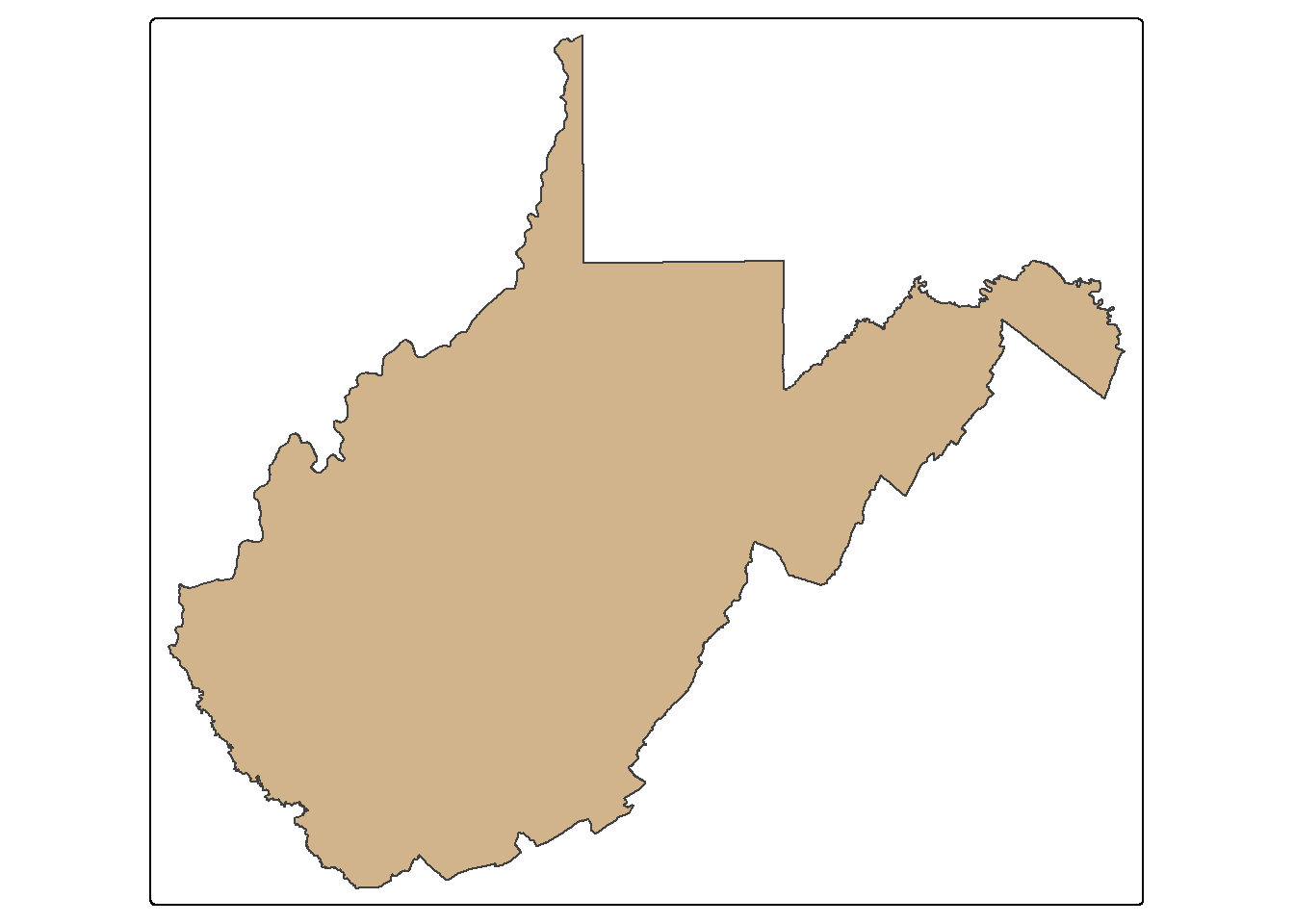
24.8.2 Proximity Analysis (Buffer)
Proximity analysis relates to finding features that are near to other features. A buffer represents the area that is within a defined distance of an input feature. Buffers can be generated for POINTS, LINES, or POLYGONS. They can also be generated for the MULTI-versions of these geometries. The result will always be a polygon or area. Below, we create polygon buffers that encompass all areas within 20 km of the mapped interstates using the st_buffer() function. The buffer distance is defined in the map units, in this case meters.
us_inter_20km <- us_inter |>
  st_buffer(20000)

tm_shape(states)+ tm_polygons(fill="tan")+
  tm_shape(us_inter_20km)+
  tm_polygons(fill="red",
              fill_alpha=.6)+
  tm_shape(us_inter)+
  tm_lines(lwd=1, col="black")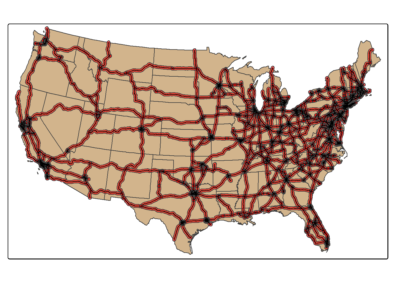
24.8.3 Vector Overlay
24.8.3.1 Intersect/Clip (AND)
Clip and intersect are used to extract features within another feature or return the overlapping extent of multiple features. Think of this as a spatial AND. When we intersect the circle and triangle, the result is the area that occurs in both the circle and the triangle (shown in red). All attributes from both features are returned, as demonstrated by calling glimpse() on the output. The table contains both the “C” and “T” fields, which came from the circle and triangle, respectively. st_intersection() is equivalent to the Intersect Tool in ArcGIS Pro. However, it can also be used to perform a clip, as the geometric result is the same.
st_intersection() and st_intersects() are sometimes confused. st_intersection() performs a spatial intersection to return a new geometry while st_intersects() is a test that returns TRUE or FALSE. It specifically tests whether two geometries or layers intersect.
isect_example <- st_intersection(circle, triangle)

tm_shape(ext)+
  tm_borders(col="black")+
  tm_shape(circle)+
  tm_polygons(fill="#0D5C86")+
  tm_shape(triangle)+
  tm_polygons(fill="#67B38C")+
  tm_shape(isect_example)+
  tm_polygons(fill="#FD694F")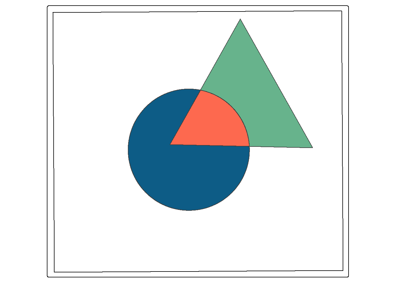
glimpse(isect_example)Rows: 1
Columns: 6
$ Id <int> 0
$ C <chr> "C"
$ Id.1 <int> 0
$ T <chr> "T"
$ area <dbl> 7360.591
$ Shape <POLYGON [m]> POLYGON ((587683.9 4395515,...In this second example, we use st_intersection(), the interstate buffers, and the tornado points to find all tornadoes that occurred within 20 km of an interstate. So, buffer and intersection can be combined to extract features within a specified distance of other features.
isect_example <- st_intersection(torn, us_inter_20km)

tm_shape(states) +
  tm_polygons(fill="tan")+
  tm_shape(us_inter_20km)+
  tm_polygons(fill="red",
              fill_alpha=.6)+
  tm_shape(us_inter)+
  tm_lines(lwd=1,
           fill="black")+
  tm_bubbles(fill="black")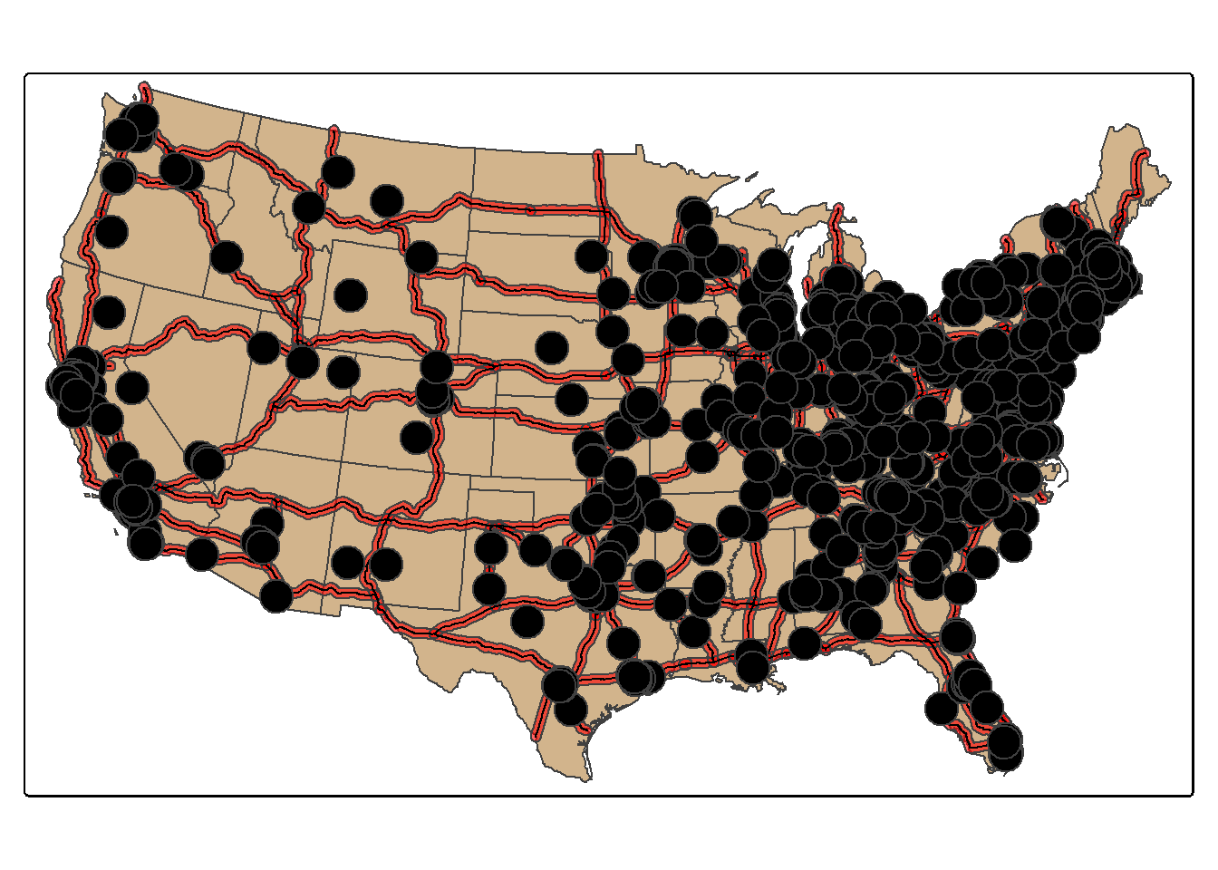
24.8.3.2 Union (OR)
st_union() from sf is a bit different from the Union Tool in ArcGIS Pro. Instead of returning the unioned area with all internal boundaries maintained, the features are merged to a single feature with no internal boundaries. In the example, the full spatial extents of the circle and triangle are returned as a single feature. Similar to st_inersection(), all attributes are maintained. Think of this as a spatial OR.
union_example <- st_union(circle, triangle, by_feature=TRUE)

tm_shape(ext)+
  tm_borders(color="black")+
  tm_shape(union_example)+
  tm_polygons(fill="#FD694F")
24.8.3.3 Difference (NOT)
st_difference() returns the portion of the the first geometric feature that is not in the second. This is similar to the Erase Tool in ArcGIS Pro. This is a spatial NOT: circle NOT triangle. The result is the portion of the circle shown by the dotted red extent displayed in the map below.
erase_example <- st_difference(circle, triangle)

tm_shape(ext)+
  tm_borders(col="black")+
  tm_shape(circle)+
  tm_polygons(fill="#0D5C86")+
  tm_shape(triangle)+
  tm_polygons(fill="#67B38C")+
  tm_shape(erase_example)+
  tm_polygons(fill="#FD694F",
              col="red",
              lty=5,
              lwd=4,
              fill_alpha=.6)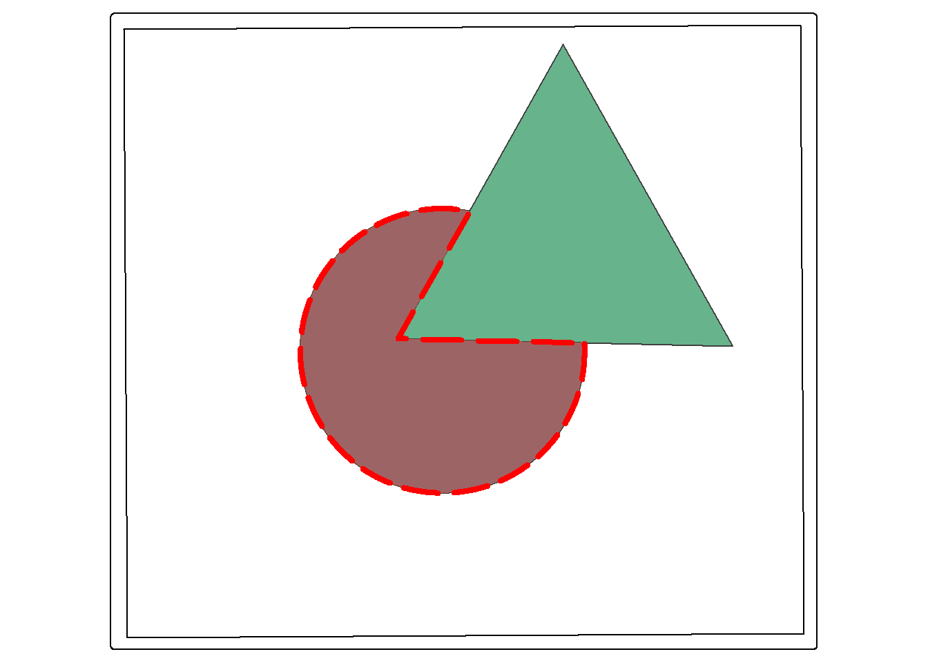
24.8.3.4 Symmetrical Difference (XOR)
Symmetrical difference is a spatial XOR: circle OR triangle, excluding circle AND triangle. So, the result is the area in either the circle or the triangle, but not the area in both.
sym_diff_examp <- st_sym_difference(circle, triangle)

tm_shape(ext)+
  tm_borders(col="black")+
  tm_shape(sym_diff_examp)+
  tm_polygons(fill="#FD694F")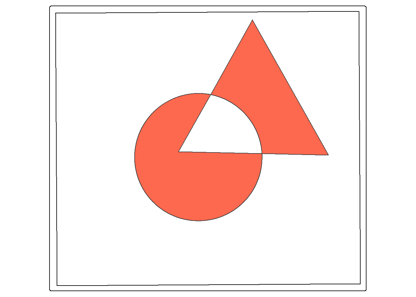
24.9 Data Summarization
24.9.1 Count Points in Polygon
You can count the number of point features occurring in polygons using sf and dplyr. The goal of the code block below is to count the number of cities in each state. This is accomplished using the following process.
- use
st_join()to join the cities and states based on spatial co-occurrence; this results in POINT geometries where each point has its original attributes plus the attributes for the state in which it occurs - use
group_by()andcount()from dplyr to count the number of cities by state - use
st_drop_geometry()to remove the geometric information from the output and return just the aspatial data - join the table back to the state boundaries using the common “STATE_NAME” field and a table join (
left_join())
Once this process is complete, we then map the resulting counts.
cities_in_state <- st_join(us_cities, states)

cities_cnt <- cities_in_state |>
  group_by(STATE_NAME) |>
  count()

cities_cnt <- st_drop_geometry(cities_cnt)

state_cnt <- left_join(states, cities_cnt, by="STATE_NAME")

tm_shape(state_cnt)+
  tm_polygons(fill="n",
              fill.legend = tm_legend(title = "Number of Cities"),
              fill.scale = tm_scale_continuous(values = "brewer.oranges"))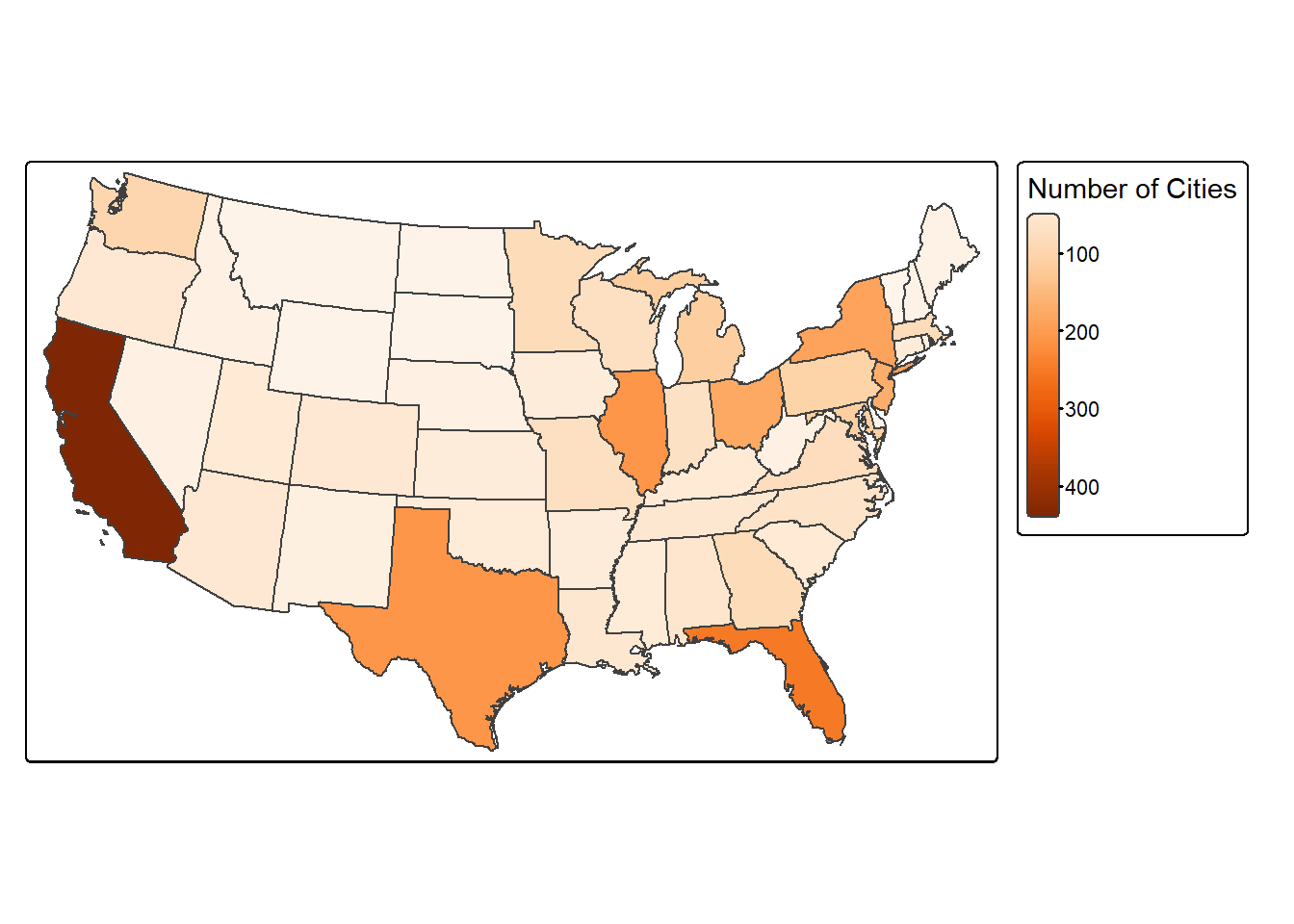
24.9.2 Length of Lines in Polygon
You can also sum the length of lines within polygons. The goal of the code below is to sum the length of interstates by state using the following process:
- intersect the interstates and states using
st_intersection()to obtain LINE geometries where the interstates have been split along state boundaries and now have the attributes for the state in which they occur - use
st_length()to calculate the length of each line segment; it is not appropriate to use the original length field because it does not reflect the length if the interstate was split along a state border; divide by 1,000 to obtain the measure in kilometers as opposed to meters - group the lines by state and sum the length using dplyr (
group_by()andsummarize()) - remove the geometry from the result (
st_drop_geometry()) - join the result back to the state boundaries using
left_join()and the common “STATE_NAME” field
us_inter_isect <- st_intersection(us_inter, states)
us_inter_isect$ln_km <- us_inter_isect |> st_length()/1000
state_ln <- us_inter_isect |>
  group_by(STATE_NAME) |>
  summarize(inter_ln = sum(ln_km)) |>
  st_drop_geometry()

state_inter_ln <- left_join(states, state_ln, by="STATE_NAME")

tm_shape(state_inter_ln)+
  tm_polygons(fill="inter_ln",
              fill.legend = tm_legend(title = "Interstate Length"),
              fill.scale = tm_scale_continuous(values = "brewer.purples"))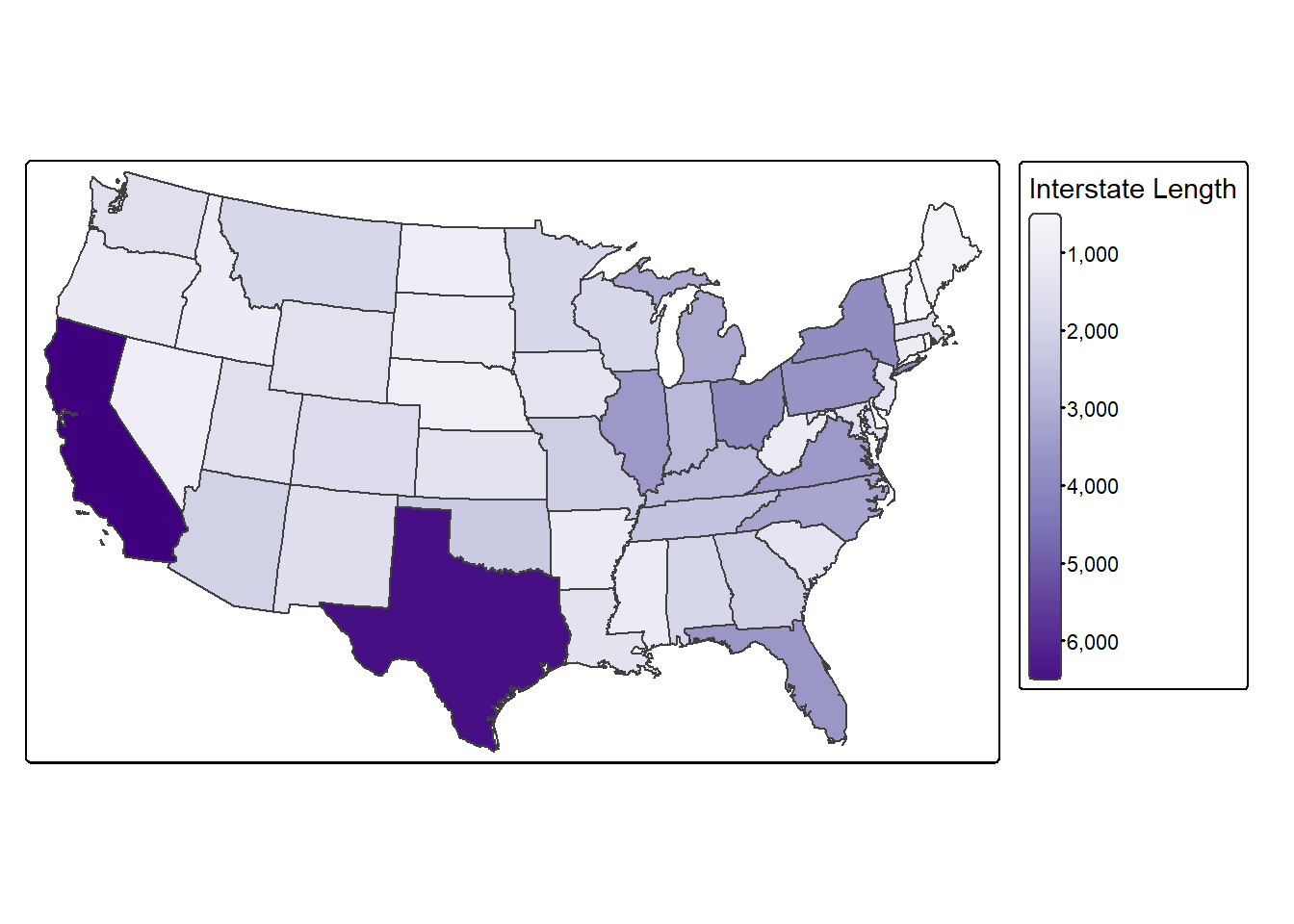
For a fairer comparison, it would make sense to calculate the density of interstates as length of interstates in kilometers per square kilometer of state area. Again, this can be accomplished using only sf and dplyr.
state_inter_ln$sq_km <- state_inter_ln |> st_area()*1e-6

state_inter_ln <- state_inter_ln |>
  mutate(int_den = inter_ln/sq_km)

tm_shape(state_inter_ln)+
  tm_polygons(fill="int_den",
              fill.legend = tm_legend(title = "km per square km"),
              fill.scale = tm_scale_intervals(style="quantile", values = "brewer.purples"))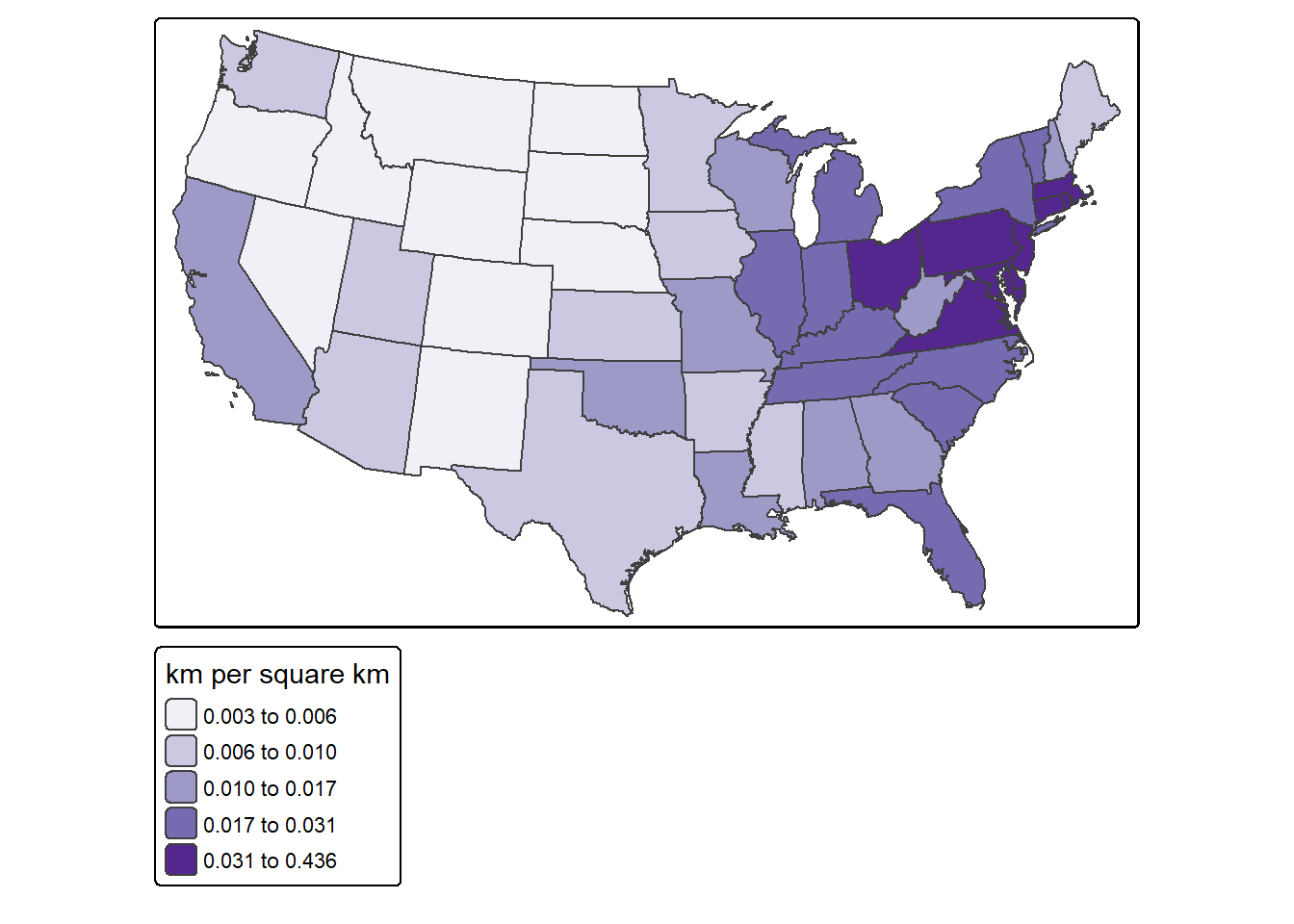
24.10 Other Operations
24.10.1 Simplify Geometry
The st_simplify() function is used to simplify or generalize features. Higher values for dTolerance result in more simplification. Topology can be preserved using the perserveTopology parameter. For simplifying the state boundaries, topology is preserved in the first example below but not the second. In the third example, a simplification of the West Virginia state boundary is generated using a tolerance of 10,000 meters with topology preserved.
state_100000 <- states |>
  st_simplify(dTolerance=100000,
              preserveTopology = TRUE)

tm_shape(state_100000)+
  tm_polygons(fill="tan")
state_100000 <- states |>
  st_simplify(dTolerance=100000, preserveTopology = FALSE)

tm_shape(state_100000)+
  tm_polygons(fill="tan")
wv_bound <- states |>
  filter(STATE_NAME=="West Virginia")|>
  st_simplify(dTolerance=10000,
              preserveTopology = TRUE)

tm_shape(wv_bound)+
  tm_polygons(fill="tan")
24.10.2 Spatial Sampling
Random points can be generated within polygons using the st_samples() function. In the example, we generate 400 random points across the country. Since this is random, a different result is obtain if the code is re-execute unless a random seed is set. You can also set the type argument to "regular" to obtain a regular as opposed to random pattern. Combining st_sample() with group_by() allows for stratify the sample based on a category. In the second example, we extract 10 random points in each state.
pnt_sample <- states |>
  st_sample(400, type="random")

tm_shape(states)+
  tm_polygons(fill="tan")+
  tm_shape(pnt_sample)+
  tm_bubbles(fill="black")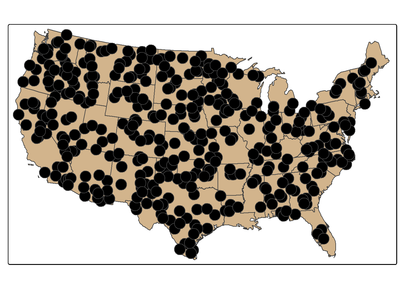
set.seed(42)
pnt_sample2 <- states |>
  group_by(STATE_NAME) |>
  st_sample(rep(10, 49), type="random")

tm_shape(states)+
  tm_polygons(fill="tan")+
  tm_shape(pnt_sample2)+
  tm_bubbles(fill="black")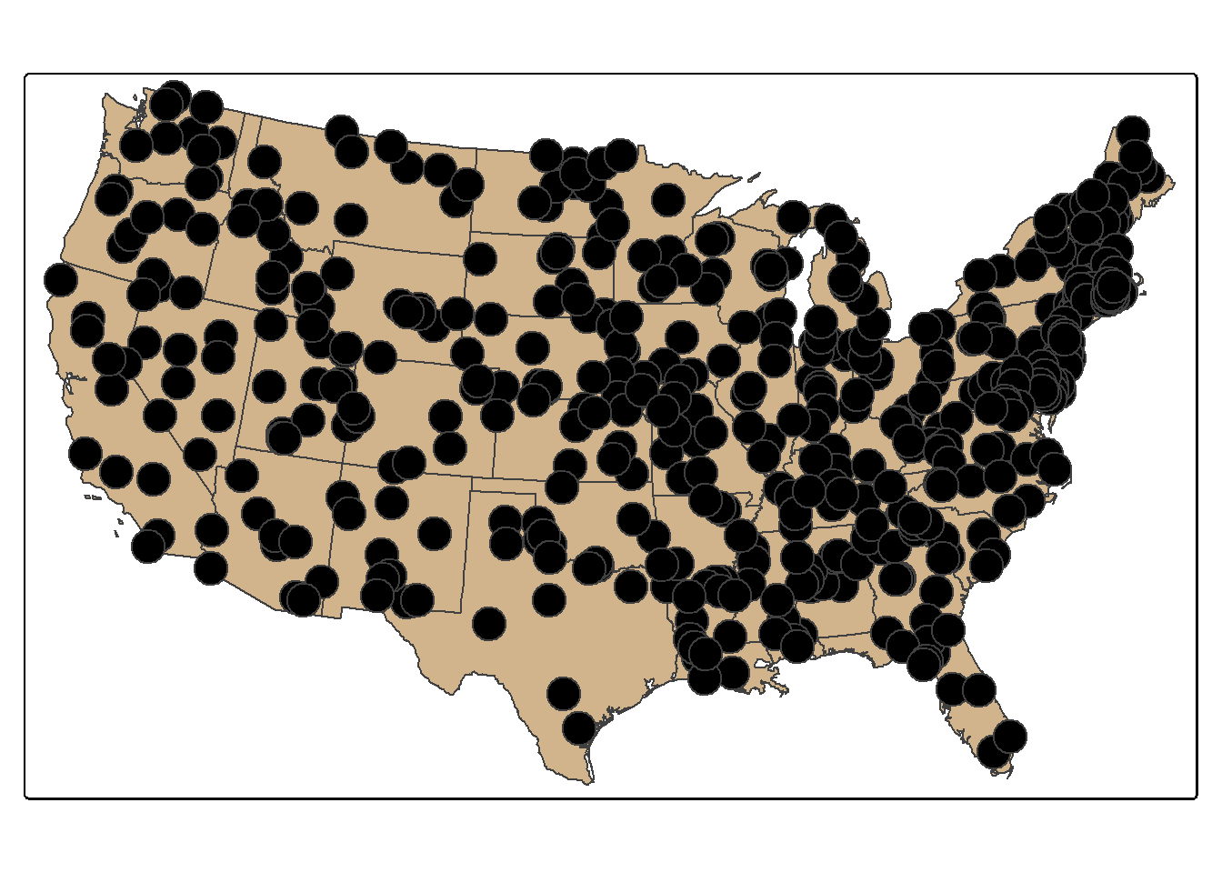
24.10.3 Tesselation
st_make_grid() can produce a rectangular grid tessellation over an extent. Below, we extract the bounding box for the states data. We then create a new grid of 10-by-10 cells within this extent using st_make_grid(). A hexagonal tessellation can be obtained by setting the square argument in st_make_grid() to FALSE.
us_grid <- states |>
  st_bbox() |>
  st_make_grid(n=c(10, 10))

tm_shape(states)+
  tm_polygons(col="tan")+
  tm_shape(us_grid)+
  tm_polygons(fill="red",
              fill_alpha=.2,
              col="black",
              lwd=2)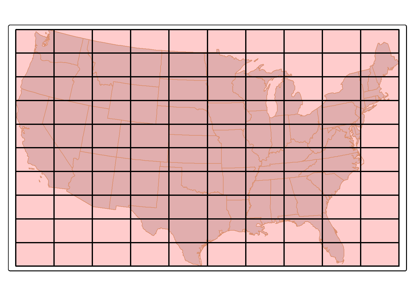
us_hex <- states |>
  st_bbox(states)|>
  st_make_grid(n=1) |>
  st_make_grid(n=c(10, 10), square=FALSE)

tm_shape(states)+
  tm_polygons(fill="tan")+
  tm_shape(us_hex)+
  tm_polygons(fill="red",
              fill_alpha=.2,
              col="black",
              lwd=2)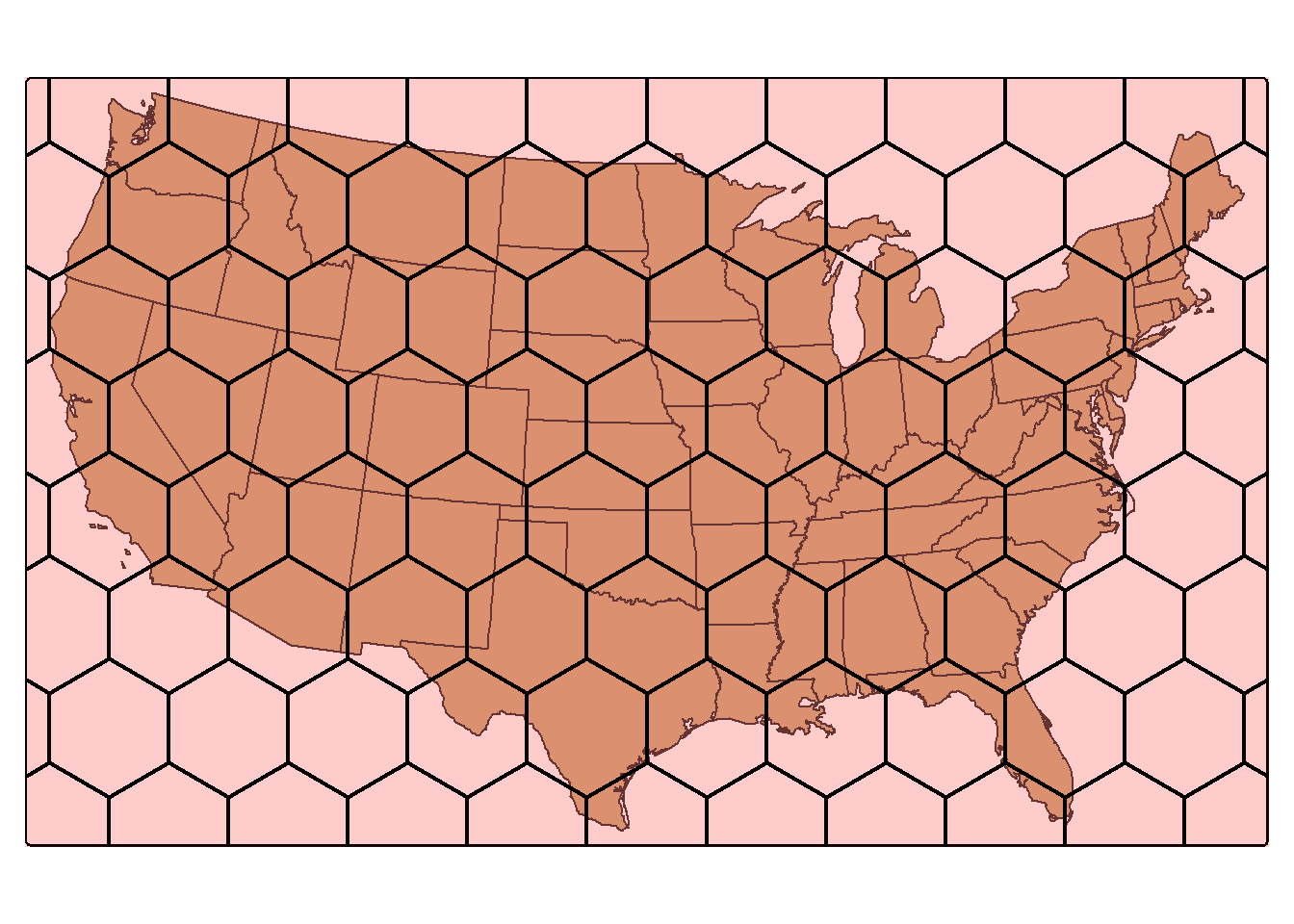
24.11 Concluding Remarks
We have tried to focus on common geoprocessing and vector analysis techniques here. You will likely run into specific issues that will require different techniques. However, we think you will find that the examples provided offer a starting point for other analyses.
24.12 Questions
- Explain the difference between
POLYGONandMULTIPOLYGONgeometries. - Explain the concept of a
GEOMETRYCOLLECTION. How is this different from other geometries? - Explain the difference between a table join, such as those implemented with dplyr, and a spatial join.
- Explain the purpose of the
dsnparameter forst_read(). - Explain the difference between
st_intersection()andst_intersects(). - Explain the difference between
st_intersection(),st_union(),st_difference(), andst_sym_difference(). - Within
st_simplify(), what is the purpose of thepreserveTopologyparameter? - Explain how you might calculate the area of polygons relative to other polygons using sf. This was not demonstrated in our examples.
24.13 Exercises
The goal of this exercise is to work with and analyze vector data in R using a wide variety of vector querying, analysis, and overlay methods and the sf package. The data layers have been provided in the exercise folder associated with the chapter and were obtained from the West Virginia GIS Technical Center.
- chpt24.gpkg/springs: point locations of springs in West Virginia
- chpt24.gpkg/towns: point locations of towns in West Virginia
- chpt24.gpkg/interstates: line features of interstates in West Virginia
- chpt24.gpkg/major_rivers: line features of major rivers in West Virginia
- chpt24.gpkg/counties: polygon features of West Virginia county boundaries
- chpt24.gpkg/geology: polygon features of geologic formations in West Virginia
Use these data layers, the tidyverse, and sf to perform the following analyses and answer the associated questions.
- Read in all of the required layers using
st_read(). - Make a map using tmap that includes the county boundaries, town points, interstates, and rivers to visualize the data.
- What percentage of towns have a population (“POPULATION”) greater than 1,500?
- How many towns are categorized as a village (use the “TYPE” field)?
- Randomly select 25 towns from the dataset.
- Randomly selection three towns from each type (use the “TYPE” field).
- What percentage of springs have an average flow (“AVEFLOW”) greater than 700?
- What percentage of springs occur on terraces (use the “TOPO_POS” field)?
- Extract out Interstate 79 from the interstate line features (use the “SIGN1” field).
- Dissolve the I-79 features to a single line feature and obtain the total length in kilometers (use the “KM” length field, which provides the length in kilometers). What is the total length?
- Extract all towns within 10 km of I-79. How many towns are within 10 km of I-79?
- Create a map using tmap to visualize the results from the analysis that includes the county boundaries, I-79 line, I-79 buffer, and the extracted town points.
- Extract all springs in limestone geology (use the “TYPE” field in the geology layer). What percent of all springs occur in limestone?
- Create a table of counts of springs by rock type. Which rock type has the largest number of springs?
- Create 5 random points per county in the state.
- Create a map using tmap to visualize the randomly sampled points that includes the county boundaries and sampled points.
- Calculate length of major rivers by county. Which county has the longest length of major rivers?
- Create a map using tmap to visualize the length of rivers by county using color.
- Calculate the density of towns by county. Which county has the largest density of towns? (note: both layers have a “NAME” field, so you will need to rename one of these fields to eliminate the overlap and confusion.)
- Create a map using tmap to visualize the density of towns by county using color.