import torch
import torch.nn
import torch.nn.functional as F9 Convolutional Neural Network Components
9.1 Introduction
The goal of this module is to explore convolutional operations and the building blocks of convolutional neural networks (CNNs) before we dive into building CNNs using PyTorch. Fortunately, CNNs, especially simple architectures, rely on a small set of building blocks. As a result, understanding these building blocks goes a long way towards understanding how CNNs work and are built.
In the code block below, I am importing torch, torch.nn, and torch.nn.functional, which is assigned the alias F. The torch.nn.functional subpackage provides functional implementations (i.e., they are coded and executed like functions) to compliment many of the class-based layers and building blocks available in PyTorch. For the demonstrations in this module, the functional implementations are much simpler to implement since I don’t have to subclass nn.Module and instantiate an instance.
9.2 2D Convolution
We will begin by building a random tensor on which to perform operations. This tensor is 4D with a shape of (1,1,9,9) and is meant to represent a tensor with the following dimensions: (mini-batch, channels, height, width). As you will see in later modules, this is a common tensor shape when feeding images into a CNN in mini-batches. I have also rescaled the random values from 0 to 1 to -1 to 1.
Next, I create another tensor that is meant to represent a kernel or moving window. This moving window has a shape of (1,1,3,3). So, it represents a single kernel that will pass over the input tensor to create a single feature map. The weights associated with this tensor would be learned during the training process to create a transformation of the input image or prior feature map that represents some useful information. However, here I am not actually building a CNN architecture or training it. Instead, I am just demonstrating convolutional operations using some random data of the correct shape. As a result, I have just filled the tensor with 1s.
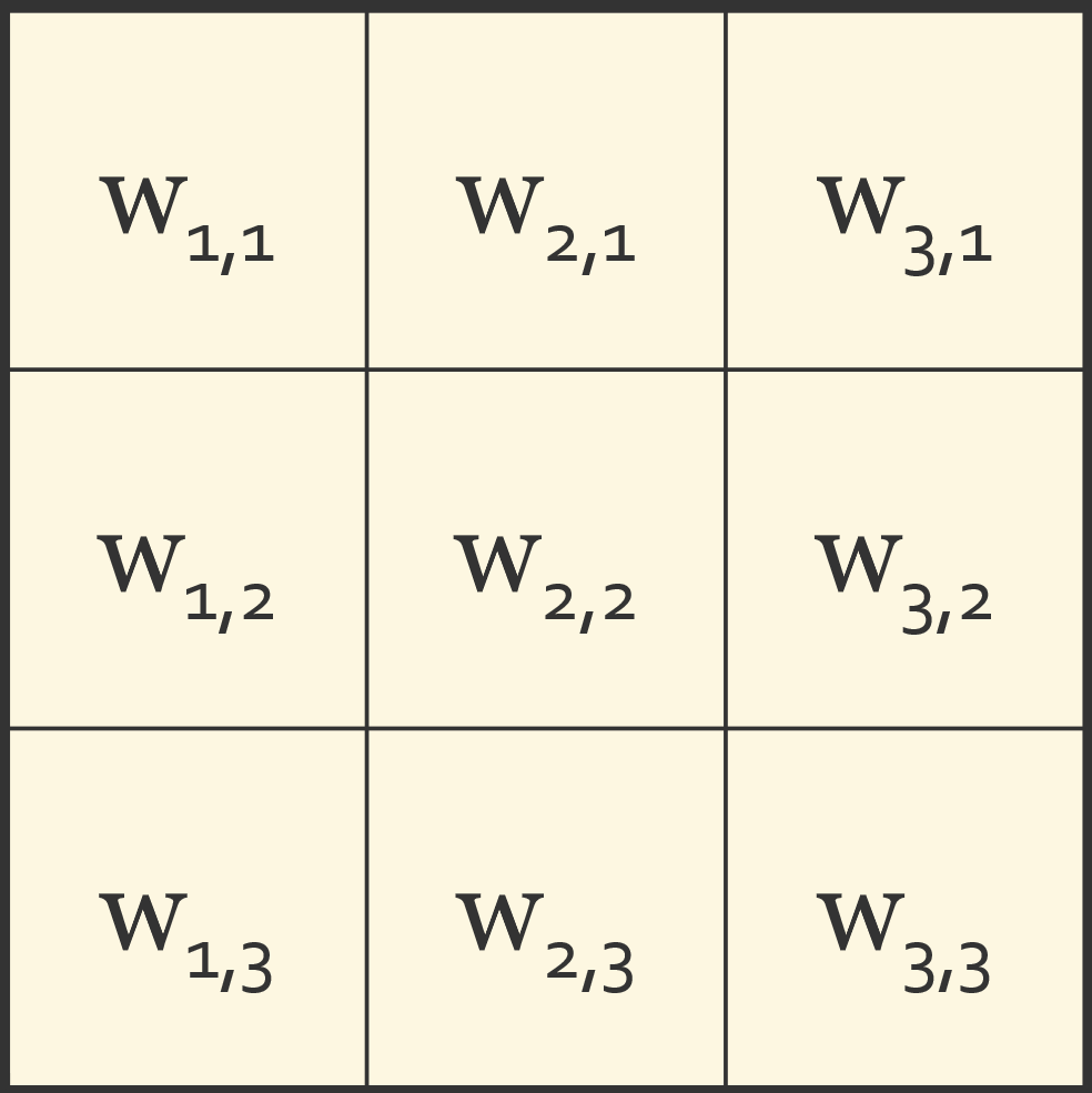
A 3x3 kernel is conceptualized in Figure 9.1. Each cell in the kernel stores a weight. As the kernel passes over the input, each weight is multiplied by the value of the cell it overlaps, the products are summed, and a bias term is added (in this demonstration, no bias is used). The result is written to the output cell corresponding to the center of the kernel. Since the same weights are applied at every location, a convolutional layer has far fewer trainable parameters than a fully connected layer that operates on the same input. If the input has multiple channels, such as the bands of a multispectral image, each kernel has a separate set of weights for each input channel, and the results for all channels are summed.
inT = (torch.rand((1,1,9,9))*2)-1
inT
tensor([[[[-0.6054, -0.5898, -0.3300, -0.7646, 0.8737, 0.2695, 0.4967,
-0.2016, 0.3609],
[-0.1009, 0.0648, -0.0550, -0.9098, -0.2369, -0.9712, 0.4491,
-0.7120, -0.1257],
[-0.6946, 0.6164, -0.5804, -0.1329, 0.9356, -0.1354, -0.0877,
0.6847, -0.5631],
[ 0.8904, -0.0698, 0.6242, 0.1351, 0.7163, -0.0373, -0.1076,
0.7424, 0.4072],
[ 0.4720, -0.5685, 0.4941, -0.3659, -0.1566, 0.2439, -0.2869,
-0.3828, 0.3678],
[ 0.6042, -0.5220, 0.5993, -0.6612, 0.0682, 0.7386, -0.2486,
0.9073, -0.1095],
[-0.7319, 0.0102, 0.0171, 0.7815, -0.9242, 0.8083, -0.6740,
0.0485, 0.0734],
[ 0.6553, -0.1942, 0.2774, -0.6153, 0.1475, 0.6823, 0.9019,
0.8486, 0.4081],
[ 0.0794, 0.5858, -0.6556, -0.3567, -0.6904, -0.7380, 0.2386,
-0.9297, -0.8912]]]])inW = torch.ones((1,1,3,3))
inWtensor([[[[1., 1., 1.],
[1., 1., 1.],
[1., 1., 1.]]]])In order to apply the kernel to the image, I use the functional version of conv2d(), which performs two-dimensional convolution. There are also functions for 1D and 3D convolution (conv1d() and conv3d()). The conv2d() function accepts an input tensor, an input kernel, and stride and padding arguments. The stride represents how much the kernel moves as it steps over the image. Since the stride is set to 1, each pixel will be placed at the center of the 3x3 kernel as it passes over the image. The padding argument is set to “same”, which indicates that padding will be added such that the height and width of the resulting feature map will be the same as the input image. Since a 3x3 kernel with a stride of 1 is being used here, “same” would yield the same result as a padding of 1.
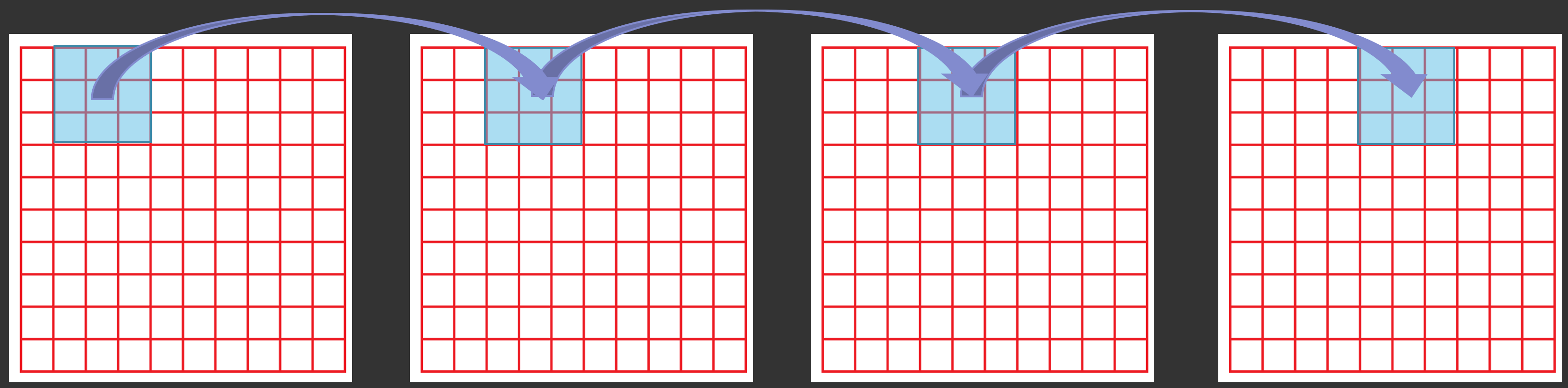
Stride is conceptualized in Figure 9.2. With a stride of 1, the kernel moves one cell at a time, so it is centered over every cell in the input. With a stride of 2, it would move two cells at a time, skipping every other cell, and the height and width of the output would be approximately halved.
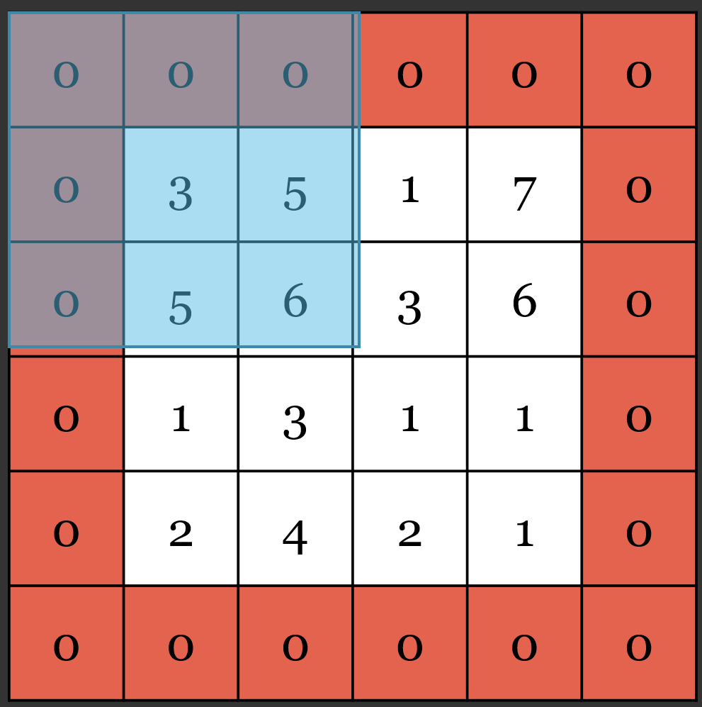
Padding is conceptualized in Figure 9.3. When the kernel is centered over a cell along the edge of the input, part of the kernel extends beyond the input. Adding a border of cells, commonly filled with zeros, allows the kernel to be centered over the edge cells, so the output has the same height and width as the input. For a 3x3 kernel, one row or column of padding is needed along each edge, and, for a 5x5 kernel, two are needed.
In the first example, the result is equivalent to adding all of the values in the 3x3 window around each cell. This is because each weight is set to 1, so each value will be multiplied by 1 then all the values will be added. In the next example, I have defined a new kernel in which only the center weight of the 3x3 kernel is 1 while all other weights are 0. This results in simply returning the center value or replicating the original values or “image”.
outT = F.conv2d(inT, inW, stride=1, padding="same")
outT
tensor([[[[-1.2313, -1.6163, -2.5843, -1.4225, -1.7393, 0.8808, -0.6695,
0.2674, -0.6783],
[-1.3095, -2.2748, -2.6812, -1.2002, -1.0720, 1.5934, -0.2079,
0.3014, -0.5567],
[ 0.7063, 0.6951, -0.3074, 0.4961, -0.6365, 0.5250, -0.1749,
0.6874, 0.4336],
[ 0.6460, 1.1838, 0.1523, 1.6695, 1.2028, 1.0843, 0.6333,
0.7741, 1.2563],
[ 0.8063, 2.5239, -0.3347, 1.4536, 0.6812, 0.9301, 1.5690,
1.2893, 1.9325],
[-0.7359, 0.3746, -0.2152, -0.1475, 0.5327, -0.4313, 1.1543,
-0.3048, 0.9047],
[-0.1784, 0.7155, -0.3071, -0.3096, 1.0258, 1.5001, 4.0130,
2.1557, 2.1764],
[ 0.4046, 0.0436, -0.1497, -2.0186, -0.9050, -0.2481, 1.1864,
0.0241, -0.4423],
[ 1.1262, 0.7481, -0.9586, -1.8931, -1.5706, 0.5419, 1.0036,
0.5763, -0.5641]]]])inW = torch.tensor([[[[0., 0., 0.],[0., 1., 0.],[0., 0., 0.]]]])
outT = F.conv2d(inT, inW, stride=1, padding="same")
outTtensor([[[[-0.6054, -0.5898, -0.3300, -0.7646, 0.8737, 0.2695, 0.4967,
-0.2016, 0.3609],
[-0.1009, 0.0648, -0.0550, -0.9098, -0.2369, -0.9712, 0.4491,
-0.7120, -0.1257],
[-0.6946, 0.6164, -0.5804, -0.1329, 0.9356, -0.1354, -0.0877,
0.6847, -0.5631],
[ 0.8904, -0.0698, 0.6242, 0.1351, 0.7163, -0.0373, -0.1076,
0.7424, 0.4072],
[ 0.4720, -0.5685, 0.4941, -0.3659, -0.1566, 0.2439, -0.2869,
-0.3828, 0.3678],
[ 0.6042, -0.5220, 0.5993, -0.6612, 0.0682, 0.7386, -0.2486,
0.9073, -0.1095],
[-0.7319, 0.0102, 0.0171, 0.7815, -0.9242, 0.8083, -0.6740,
0.0485, 0.0734],
[ 0.6553, -0.1942, 0.2774, -0.6153, 0.1475, 0.6823, 0.9019,
0.8486, 0.4081],
[ 0.0794, 0.5858, -0.6556, -0.3567, -0.6904, -0.7380, 0.2386,
-0.9297, -0.8912]]]])print(inT.shape)torch.Size([1, 1, 9, 9])print(outT.shape)torch.Size([1, 1, 9, 9])As the code blocks above demonstrate, when padding is set to “same” the height and width of the resulting feature map will be the same as the input image or tensor. If the padding is set to 0, no padding will be added, and only cells that have a full set of neighbors within a 3x3 window will be processed. This will result in dropping the outer most rows and columns to yield a tensor that has a height and width of 7x7 as opposed to 9x9.
inW = torch.tensor([[[[0., 0., 0.],[0., 1., 0.],[0., 0., 0.]]]])
outT = F.conv2d(inT, inW, stride=1, padding=0)
outT
tensor([[[[ 0.0648, -0.0550, -0.9098, -0.2369, -0.9712, 0.4491, -0.7120],
[ 0.6164, -0.5804, -0.1329, 0.9356, -0.1354, -0.0877, 0.6847],
[-0.0698, 0.6242, 0.1351, 0.7163, -0.0373, -0.1076, 0.7424],
[-0.5685, 0.4941, -0.3659, -0.1566, 0.2439, -0.2869, -0.3828],
[-0.5220, 0.5993, -0.6612, 0.0682, 0.7386, -0.2486, 0.9073],
[ 0.0102, 0.0171, 0.7815, -0.9242, 0.8083, -0.6740, 0.0485],
[-0.1942, 0.2774, -0.6153, 0.1475, 0.6823, 0.9019, 0.8486]]]])print(inT.shape)torch.Size([1, 1, 9, 9])print(outT.shape)torch.Size([1, 1, 7, 7])It is also possible to apply multiple kernels to an input. Below, I am creating 3 3x3 kernels, all filled with weights of 1. When these kernels are applied to the input tensor, three feature maps are generated.
inW = torch.ones((3,1,3,3))
outT = F.conv2d(inT, inW, stride=1, padding="same")
outT
tensor([[[[-1.2313, -1.6163, -2.5843, -1.4225, -1.7393, 0.8808, -0.6695,
0.2674, -0.6783],
[-1.3095, -2.2748, -2.6812, -1.2002, -1.0720, 1.5934, -0.2079,
0.3014, -0.5567],
[ 0.7063, 0.6951, -0.3074, 0.4961, -0.6365, 0.5250, -0.1749,
0.6874, 0.4336],
[ 0.6460, 1.1838, 0.1523, 1.6695, 1.2028, 1.0843, 0.6333,
0.7741, 1.2563],
[ 0.8063, 2.5239, -0.3347, 1.4536, 0.6812, 0.9301, 1.5690,
1.2893, 1.9325],
[-0.7359, 0.3746, -0.2152, -0.1475, 0.5327, -0.4313, 1.1543,
-0.3048, 0.9047],
[-0.1784, 0.7155, -0.3071, -0.3096, 1.0258, 1.5001, 4.0130,
2.1557, 2.1764],
[ 0.4046, 0.0436, -0.1497, -2.0186, -0.9050, -0.2481, 1.1864,
0.0241, -0.4423],
[ 1.1262, 0.7481, -0.9586, -1.8931, -1.5706, 0.5419, 1.0036,
0.5763, -0.5641]],
[[-1.2313, -1.6163, -2.5843, -1.4225, -1.7393, 0.8808, -0.6695,
0.2674, -0.6783],
[-1.3095, -2.2748, -2.6812, -1.2002, -1.0720, 1.5934, -0.2079,
0.3014, -0.5567],
[ 0.7063, 0.6951, -0.3074, 0.4961, -0.6365, 0.5250, -0.1749,
0.6874, 0.4336],
[ 0.6460, 1.1838, 0.1523, 1.6695, 1.2028, 1.0843, 0.6333,
0.7741, 1.2563],
[ 0.8063, 2.5239, -0.3347, 1.4536, 0.6812, 0.9301, 1.5690,
1.2893, 1.9325],
[-0.7359, 0.3746, -0.2152, -0.1475, 0.5327, -0.4313, 1.1543,
-0.3048, 0.9047],
[-0.1784, 0.7155, -0.3071, -0.3096, 1.0258, 1.5001, 4.0130,
2.1557, 2.1764],
[ 0.4046, 0.0436, -0.1497, -2.0186, -0.9050, -0.2481, 1.1864,
0.0241, -0.4423],
[ 1.1262, 0.7481, -0.9586, -1.8931, -1.5706, 0.5419, 1.0036,
0.5763, -0.5641]],
[[-1.2313, -1.6163, -2.5843, -1.4225, -1.7393, 0.8808, -0.6695,
0.2674, -0.6783],
[-1.3095, -2.2748, -2.6812, -1.2002, -1.0720, 1.5934, -0.2079,
0.3014, -0.5567],
[ 0.7063, 0.6951, -0.3074, 0.4961, -0.6365, 0.5250, -0.1749,
0.6874, 0.4336],
[ 0.6460, 1.1838, 0.1523, 1.6695, 1.2028, 1.0843, 0.6333,
0.7741, 1.2563],
[ 0.8063, 2.5239, -0.3347, 1.4536, 0.6812, 0.9301, 1.5690,
1.2893, 1.9325],
[-0.7359, 0.3746, -0.2152, -0.1475, 0.5327, -0.4313, 1.1543,
-0.3048, 0.9047],
[-0.1784, 0.7155, -0.3071, -0.3096, 1.0258, 1.5001, 4.0130,
2.1557, 2.1764],
[ 0.4046, 0.0436, -0.1497, -2.0186, -0.9050, -0.2481, 1.1864,
0.0241, -0.4423],
[ 1.1262, 0.7481, -0.9586, -1.8931, -1.5706, 0.5419, 1.0036,
0.5763, -0.5641]]]])If a stride greater than 1 is used, the size of the resulting array in the spatial dimensions will decrease in comparison to the input since the kernel will not be centered over each cell but will skip cells. This is one means to decrease the size of the spatial dimensions of an array. However, this is not commonly used. Instead, pooling operations are applied, which will be discussed below. When building CNNs, we will generally use a stride of 1. However, there are some applications where other strides are used. For example, when we discuss the ResNet architecture, you will see that it uses a stride of 2 as a means to decrease the size of the arrays at certain points in the network architecture.
inW = torch.ones((1,1,3,3))
outT = F.conv2d(inT, inW, stride=2)
outT
tensor([[[[-2.2748, -1.2002, 1.5934, 0.3014],
[ 1.1838, 1.6695, 1.0843, 0.7741],
[ 0.3746, -0.1475, -0.4313, -0.3048],
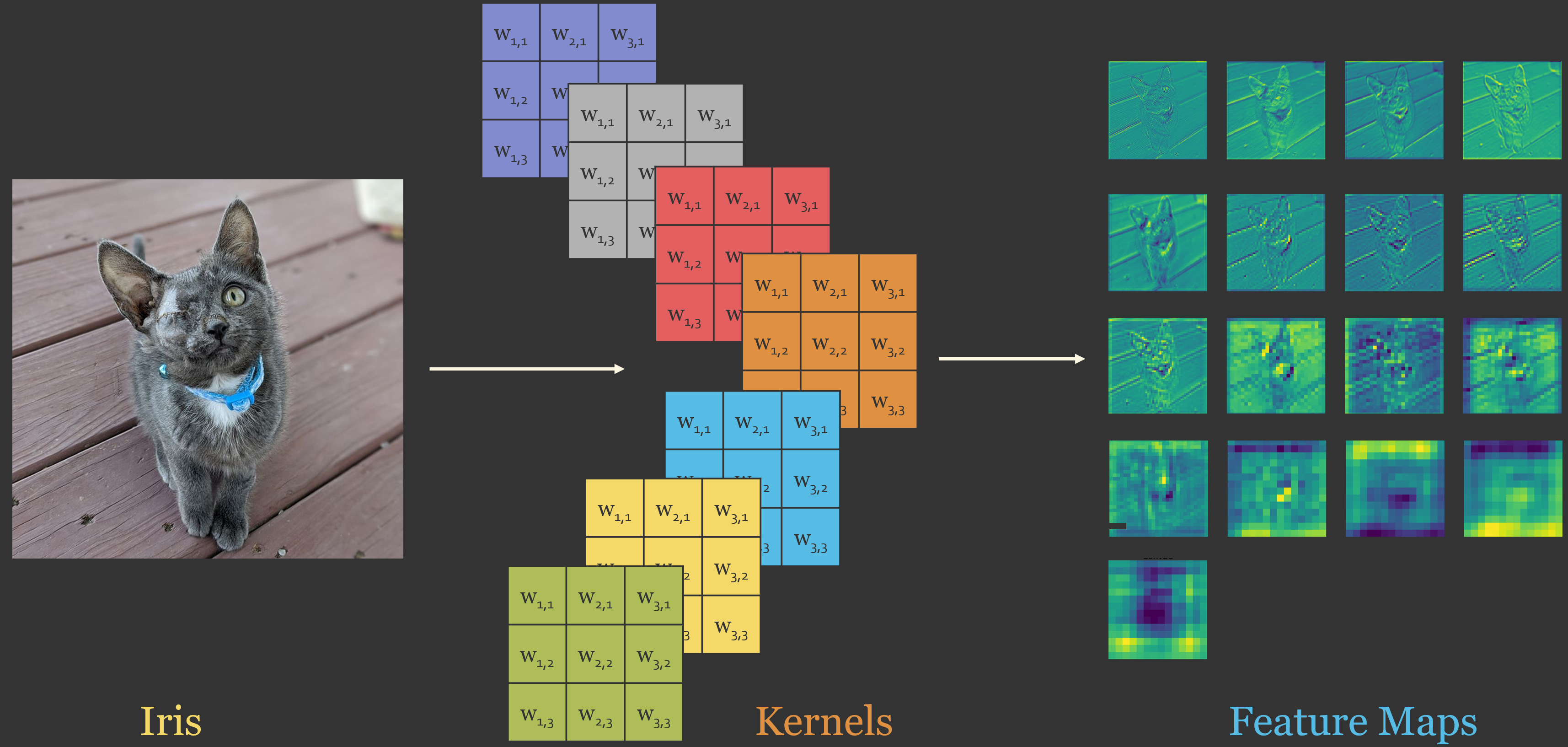
[ 0.0436, -2.0186, -0.2481, 0.0241]]]])print(inT.shape)torch.Size([1, 1, 9, 9])print(outT.shape)torch.Size([1, 1, 4, 4])The output of applying a kernel to an input is called a feature map. Each kernel in a convolutional layer generates its own feature map, so a layer with 64 kernels generates 64 feature maps, which are stacked as channels and passed to the next layer. Since the kernel weights are learned during training, each kernel learns to highlight a different pattern in the input. Figure 9.4 shows example feature maps generated from a photograph of my cat, Iris. The feature maps generated by the early layers of a CNN, shown in the top rows, highlight low-level features, such as edges and textures, and they look similar to the input image. Deeper in the network, after the spatial dimensions have been reduced, the feature maps, shown in the bottom rows, have coarser spatial resolution and represent more abstract features that are more difficult to interpret visually but are useful for differentiating classes. This hierarchical learning of increasingly abstract features is what makes CNNs so effective for image analysis.
9.3 Pooling
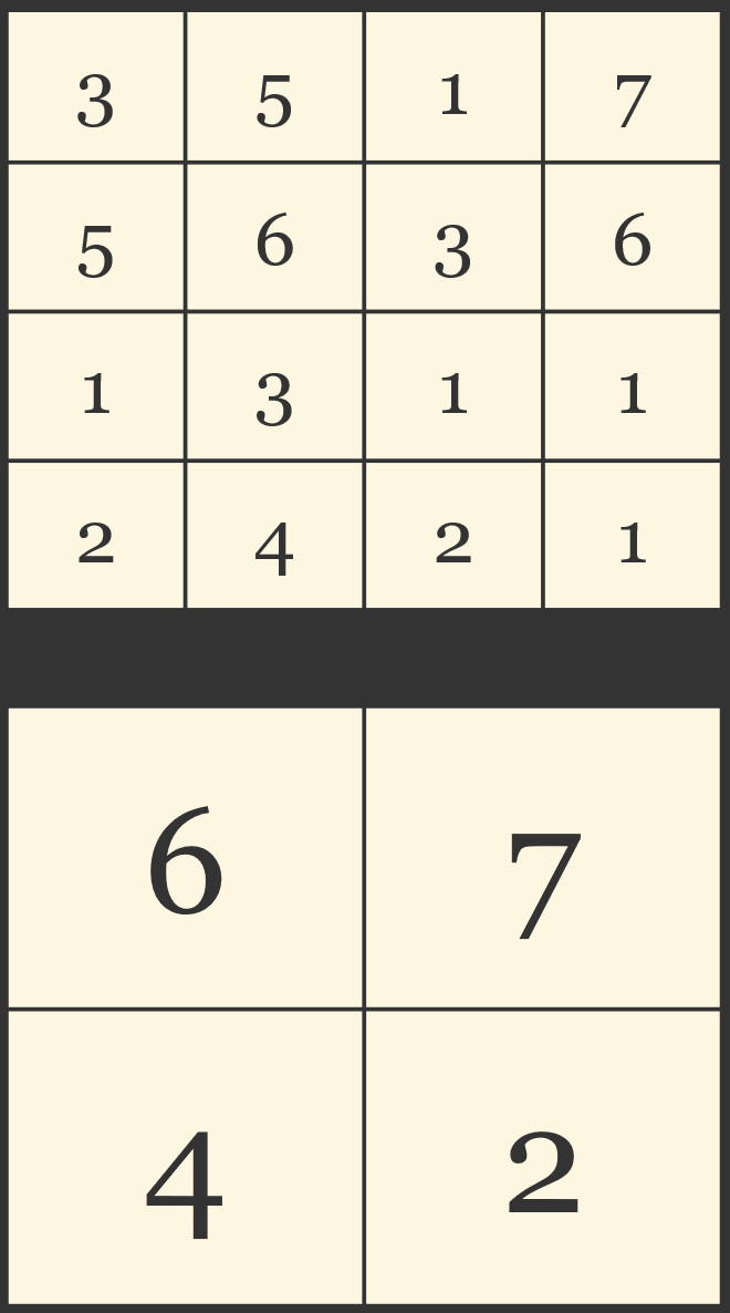
In CNN architectures, pooling operations are commonly used to decrease the size of the array in the spatial dimensions as opposed to accomplishing this by increasing the stride in the convolution operations. The most commonly used pooling operation is max pooling, which is demonstrated below. Here, an input tensor with a shape of (1,1,10,10) is transformed to a shape of (1,1,5,5) using max pooling. This is a very simple operation. In a 2x2 window, the largest or maximum value is returned. You can see that the max_pool2d() function accepts an input tensor, a window size, and a stride. By using a window size of 2x2, I essentially combine 4 cells to a single cell by returning the maximum value of the 4 values. When using a stride of 2, there is no overlap between the 2x2 windows. This process is shown in Figure 9.5. Note that max pooling has no trainable parameters.
inT = (torch.rand((1,1,10,10))*2)-1
inT
tensor([[[[-0.5005, 0.0696, -0.0105, -0.6791, -0.3055, 0.5895, -0.9830,
0.3038, -0.9535, 0.4702],
[ 0.1733, -0.8490, 0.4544, 0.9535, -0.6612, -0.7186, 0.1475,
-0.3829, 0.5761, -0.8448],
[-0.0452, -0.2416, 0.4114, 0.7990, -0.5665, 0.5357, 0.8296,
0.9869, -0.7616, 0.3838],
[ 0.5329, 0.2123, -0.6317, -0.1713, -0.9696, -0.6937, 0.7289,
-0.4098, 0.7580, 0.4808],
[-0.8361, -0.3910, 0.5420, 0.4984, -0.8335, 0.7376, -0.4029,
0.8449, 0.7126, -0.6332],
[ 0.5759, -0.8364, 0.2015, -0.8352, -0.0849, -0.1710, 0.2764,
-0.4831, -0.4187, -0.4185],
[-0.2139, 0.0685, -0.6820, -0.8529, -0.1698, 0.4700, 0.3941,
-0.9424, -0.8396, -0.0411],
[-0.5897, 0.1745, 0.8230, -0.0082, -0.7996, -0.4013, -0.7524,
0.0575, -0.3196, 0.2315],
[ 0.0362, 0.7175, -0.4482, -0.7200, 0.4138, 0.9836, 0.9512,
-0.3668, 0.2867, 0.9876],
[-0.0155, 0.7216, -0.3554, 0.7703, 0.8718, 0.9434, -0.0247,
0.3248, 0.1898, -0.6329]]]])outT = F.max_pool2d(inT, (2,2), stride=2)
outTtensor([[[[0.1733, 0.9535, 0.5895, 0.3038, 0.5761],
[0.5329, 0.7990, 0.5357, 0.9869, 0.7580],
[0.5759, 0.5420, 0.7376, 0.8449, 0.7126],
[0.1745, 0.8230, 0.4700, 0.3941, 0.2315],
[0.7216, 0.7703, 0.9836, 0.9512, 0.9876]]]])print(inT.shape)torch.Size([1, 1, 10, 10])print(outT.shape)torch.Size([1, 1, 5, 5])Although there are other pooling operations, max pooling tends to be used most often. This is because the maximum value in the window is generally associated with the most defining feature or the largest activation. However, this is just a simple interpretation and may not hold true in all cases.
Below, I demonstrate another pooling operation: average pooling. This is the same as max pooling except that the average is returned as opposed to the maximum. You will see this applied when we discuss ResNet.
Similar to convolutional operations, there are 1D and 3D versions of pooling operations.
outT = F.avg_pool2d(inT, (2,2), stride=2)
outT
tensor([[[[-0.2766, 0.1796, -0.2740, -0.2286, -0.1880],
[ 0.1146, 0.1018, -0.4235, 0.5339, 0.2152],
[-0.3719, 0.1017, -0.0880, 0.0588, -0.1894],
[-0.1401, -0.1800, -0.2252, -0.3108, -0.2422],
[ 0.3649, -0.1884, 0.8032, 0.2211, 0.2078]]]])9.4 Activation Functions
One of the issues with only applying convolution operations or fully connected layers is that this only allows for linear transformations of values. In order to introduce non-linearity into the CNN, we need to incorporate activation functions. Below, I have implemented a few activation functions. Currently, one of the most commonly used activation functions is the rectified linear unit (ReLU). This is an operation that simply converts any negative values to 0 and does not alter any positive values. Leaky ReLU is an alternative version of ReLU that maintains negative values but reduces their magnitude using a slope term. This is sometimes useful to combat the “dying ReLU” problem.
Some activation functions have an inplace parameter, which allows you to modify the values in place as opposed to saving the result to a new location in memory.
inT = torch.rand(1,2,5,5)*2-1
inT
tensor([[[[ 0.1863, -0.4417, 0.1305, 0.5154, 0.5106],
[ 0.5736, -0.9441, -0.7622, -0.8769, 0.2678],
[-0.4622, 0.9725, -0.8426, 0.1907, 0.6794],
[ 0.3797, -0.4966, -0.4889, -0.4622, -0.3597],
[ 0.7940, 0.9393, -0.8762, -0.6604, -0.8614]],
[[ 0.2119, -0.2863, 0.0864, -0.5431, 0.9014],
[ 0.5092, 0.3762, 0.2878, 0.5917, 0.8846],
[ 0.9012, 0.5750, 0.2456, -0.0748, -0.5577],
[ 0.0476, 0.9622, -0.3832, -0.6020, 0.4958],
[ 0.2855, 0.0350, -0.6320, 0.4404, -0.0524]]]])outT = F.relu(inT)
outTtensor([[[[0.1863, 0.0000, 0.1305, 0.5154, 0.5106],
[0.5736, 0.0000, 0.0000, 0.0000, 0.2678],
[0.0000, 0.9725, 0.0000, 0.1907, 0.6794],
[0.3797, 0.0000, 0.0000, 0.0000, 0.0000],
[0.7940, 0.9393, 0.0000, 0.0000, 0.0000]],
[[0.2119, 0.0000, 0.0864, 0.0000, 0.9014],
[0.5092, 0.3762, 0.2878, 0.5917, 0.8846],
[0.9012, 0.5750, 0.2456, 0.0000, 0.0000],
[0.0476, 0.9622, 0.0000, 0.0000, 0.4958],
[0.2855, 0.0350, 0.0000, 0.4404, 0.0000]]]])outT = F.leaky_relu(inT, negative_slope=.1)
outTtensor([[[[ 0.1863, -0.0442, 0.1305, 0.5154, 0.5106],
[ 0.5736, -0.0944, -0.0762, -0.0877, 0.2678],
[-0.0462, 0.9725, -0.0843, 0.1907, 0.6794],
[ 0.3797, -0.0497, -0.0489, -0.0462, -0.0360],
[ 0.7940, 0.9393, -0.0876, -0.0660, -0.0861]],
[[ 0.2119, -0.0286, 0.0864, -0.0543, 0.9014],
[ 0.5092, 0.3762, 0.2878, 0.5917, 0.8846],
[ 0.9012, 0.5750, 0.2456, -0.0075, -0.0558],
[ 0.0476, 0.9622, -0.0383, -0.0602, 0.4958],
[ 0.2855, 0.0350, -0.0632, 0.4404, -0.0052]]]])The sigmoid activation function can be used to convert values to a range between 0 and 1. This is a common activation function applied after the last linear layer in a fully connected neural network or a CNN that is performing a binary classification. For binary classification, the last fully connected layer will have an output size of 1. The raw logits can be passed through a sigmoid activation function in order to scale them from 0 to 1. In the example below, I generate a 1D array of logits representing results for four separate data points. Each data point is then rescaled separately, or element-wise, using the sigmoid function to be between 0 and 1.
inT = torch.tensor([4.1, -1.1, 3.3, 2.2])
print(torch.sigmoid(inT))
tensor([0.9837, 0.2497, 0.9644, 0.9002])For multiclass classification, a softmax activation is commonly used instead of a sigmoid activation. When performing a multiclass classification, the last layer will output one node for each class. As a result, raw logits will be returned for each class, and the prediction will correspond to the class with the highest logit. In order to convert these raw logits to probabilities that sum to 1, the softmax activation is applied. This requires defining a dimension over which the probabilities should sum to 1. In the example, the 2nd dimension (i.e., index 1) represents all the predicted logits for a single observation.
inT = torch.tensor([[4.1, -1.1, 3.3, 2.2], [3.6, 2.3, -0.5, -1.2], [1.7, 3.3, .7, .2]])
print(torch.softmax(inT, dim=1))
tensor([[0.6233, 0.0034, 0.2801, 0.0932],
[0.7708, 0.2101, 0.0128, 0.0063],
[0.1528, 0.7569, 0.0562, 0.0341]])It should be noted that some loss functions may expect raw logits while others may expect the data to be passed through a sigmoid or softmax activation beforehand. Here are a few tips.
nn.CrossEntropyLoss()for multiclass problems expects logitsnn.NLLLoss()for multiclass problems expects probabilitiesnn.BCELoss()for binary classification expects probabilitiesnn.BCEWithLogitsLoss()for binary classification expects logits (this combines the sigmoid and BCE loss operations)
Given the above tips, when using PyTorch for a multiclass classification, I generally do not incorporate a softmax activation at the end of the network if I am using cross entropy loss since the PyTorch implementation of this loss metric expects raw logits. If you are using an alternative loss metric, such as Dice or Tversky, you will need to investigate the implementation and make sure you are providing it with the expected data: either raw logits or probabilities (i.e., logits have been passed through a softmax activation).
For binary classification and if you use nn.BCELoss(), you must pass the logits through a sigmoid activation beforehand. If you use nn.BCEWithLogitsLoss(), you should provide the raw logits since this loss incorporates the sigmoid activation. If you are using an alternative loss metric, such as Dice or Tversky, you will need to explore the implementation and make sure you are providing it with the expected data: either raw logits or probabilities (i.e., logits have been passed through a sigmoid activation).
Finally, it is possible to treat any binary classification problem as a multiclass classification problem in which the last layer outputs two logits, one for each class, as opposed to one for the positive case. If you treat a binary classification problem the same as a multiclass classification problem, then you would want to make use of nn.CrossEntropyLoss(). If you use a loss that expects probabilities, you would want to use softmax as opposed to a sigmoid activation.
9.5 Deconvolution and Upsampling
For regular CNNs in which the goal is to perform labeling of an entire image as opposed to labeling or predicting each individual pixel in the image, deconvolution is not required. However, when performing pixel-level classification (i.e., semantic segmentation) or regression the decoder component must have a means to scale up the feature maps in the spatial dimensions in order to regenerate the original spatial dimensions of the scene.
This upscaling or upsampling can be performed using a couple of different methods. The interpolate() function (named upsample() in older versions of PyTorch) operates similarly to resampling methods that we use in the geospatial sciences. New cell values are estimated using nearby original values mathematically with an interpolation method, such as nearest neighbor, bilinear, or bicubic. This form of upsampling is not really deconvolution since no kernels and associated weights are being applied.
As examples below, I have performed upsampling on a tensor with spatial dimensions of 4x4 using the nearest neighbor and bilinear interpolation methods. When using nearest neighbor, the nearest cell value is used, and you can see that values have been replicated in the result. In contrast, bilinear interpolation performs a inverse distance-weighted averaging of the 4 nearest original cells to the output cell.
inT = torch.rand(1,2,4,4)*2-1
inT
tensor([[[[ 0.4503, 0.0833, -0.6965, 0.8228],
[-0.8214, 0.8908, 0.6156, 0.4026],
[ 0.0118, 0.3146, -0.1843, -0.3020],
[ 0.3910, 0.7525, 0.3148, 0.4706]],
[[-0.7241, -0.3974, 0.3352, 0.4076],
[-0.8810, 0.5415, 0.1004, 0.2843],
[-0.4944, 0.2421, 0.4414, -0.4244],
[-0.1388, -0.6546, -0.4288, 0.7797]]]])outT = F.interpolate(inT, size=(8,8), mode="nearest")
outTtensor([[[[ 0.4503, 0.4503, 0.0833, 0.0833, -0.6965, -0.6965, 0.8228,
0.8228],
[ 0.4503, 0.4503, 0.0833, 0.0833, -0.6965, -0.6965, 0.8228,
0.8228],
[-0.8214, -0.8214, 0.8908, 0.8908, 0.6156, 0.6156, 0.4026,
0.4026],
[-0.8214, -0.8214, 0.8908, 0.8908, 0.6156, 0.6156, 0.4026,
0.4026],
[ 0.0118, 0.0118, 0.3146, 0.3146, -0.1843, -0.1843, -0.3020,
-0.3020],
[ 0.0118, 0.0118, 0.3146, 0.3146, -0.1843, -0.1843, -0.3020,
-0.3020],
[ 0.3910, 0.3910, 0.7525, 0.7525, 0.3148, 0.3148, 0.4706,
0.4706],
[ 0.3910, 0.3910, 0.7525, 0.7525, 0.3148, 0.3148, 0.4706,
0.4706]],
[[-0.7241, -0.7241, -0.3974, -0.3974, 0.3352, 0.3352, 0.4076,
0.4076],
[-0.7241, -0.7241, -0.3974, -0.3974, 0.3352, 0.3352, 0.4076,
0.4076],
[-0.8810, -0.8810, 0.5415, 0.5415, 0.1004, 0.1004, 0.2843,
0.2843],
[-0.8810, -0.8810, 0.5415, 0.5415, 0.1004, 0.1004, 0.2843,
0.2843],
[-0.4944, -0.4944, 0.2421, 0.2421, 0.4414, 0.4414, -0.4244,
-0.4244],
[-0.4944, -0.4944, 0.2421, 0.2421, 0.4414, 0.4414, -0.4244,
-0.4244],
[-0.1388, -0.1388, -0.6546, -0.6546, -0.4288, -0.4288, 0.7797,
0.7797],
[-0.1388, -0.1388, -0.6546, -0.6546, -0.4288, -0.4288, 0.7797,
0.7797]]]])outT = F.interpolate(inT, size=(8,8), mode="bilinear")
outTtensor([[[[ 0.4503, 0.3585, 0.1751, -0.1116, -0.5016, -0.3167, 0.4430,
0.8228],
[ 0.1324, 0.1706, 0.2470, 0.1218, -0.2051, -0.0969, 0.4462,
0.7178],
[-0.5035, -0.2054, 0.3909, 0.5886, 0.3879, 0.3426, 0.4526,
0.5077],
[-0.6131, -0.2731, 0.4068, 0.6640, 0.4984, 0.3683, 0.2738,
0.2265],
[-0.1965, -0.0327, 0.2949, 0.3479, 0.1265, -0.0197, -0.0904,
-0.1258],
[ 0.1066, 0.1860, 0.3447, 0.3032, 0.0614, -0.0718, -0.0965,
-0.1088],
[ 0.2962, 0.3829, 0.5563, 0.5298, 0.3033, 0.2119, 0.2556,
0.2775],
[ 0.3910, 0.4814, 0.6621, 0.6430, 0.4242, 0.3538, 0.4317,
0.4706]],
[[-0.7241, -0.6424, -0.4791, -0.2142, 0.1520, 0.3533, 0.3895,
0.4076],
[-0.7633, -0.6132, -0.3128, -0.0529, 0.1667, 0.3015, 0.3517,
0.3768],
[-0.8418, -0.5546, 0.0197, 0.2699, 0.1960, 0.1981, 0.2761,
0.3151],
[-0.7844, -0.4716, 0.1539, 0.3964, 0.2559, 0.1660, 0.1267,
0.1071],
[-0.5910, -0.3640, 0.0899, 0.3267, 0.3463, 0.2053, -0.0964,
-0.2473],
[-0.4055, -0.2996, -0.0879, 0.0694, 0.1724, 0.1370, -0.0366,
-0.1234],
[-0.2277, -0.2784, -0.3798, -0.3757, -0.2661, -0.0388, 0.3062,
0.4787],
[-0.1388, -0.2677, -0.5257, -0.5982, -0.4853, -0.1267, 0.4776,
0.7797]]]])As noted above, the upsampling method is not a convolutional, or “deconvolutional”, operation since no kernels are applied. Since there are no kernels and associated weights, there are no trainable parameters associated with upsampling.
The conv_transpose2d() function, or the nn.ConvTranspose2d() layer, allows for upsampling a tensor in the spatial dimensions using kernels that have trainable weights. If transpose convolution is applied with a kernel size of 2x2 and a stride of 2 then this will result in doubling the size of the tensor in the spatial dimensions. Practically, this operation can return the original tensor spatial dimensions before max pooling with a 2x2 kernel and a stride of 2 was applied. To be clear, 2D transpose does not undo prior convolutional operations. Instead, it learns new weights as it scales up the data.
Transpose convolution is conceptualized in Figure 9.6. Each input cell is multiplied by the 2x2 kernel to generate a 2x2 block of predicted values in the output, so the output has twice the height and width of the input. This is equivalent to inserting cells between the original cells, adding padding around the edges, and passing the 2x2 kernel over the resulting array, as shown in the figure.
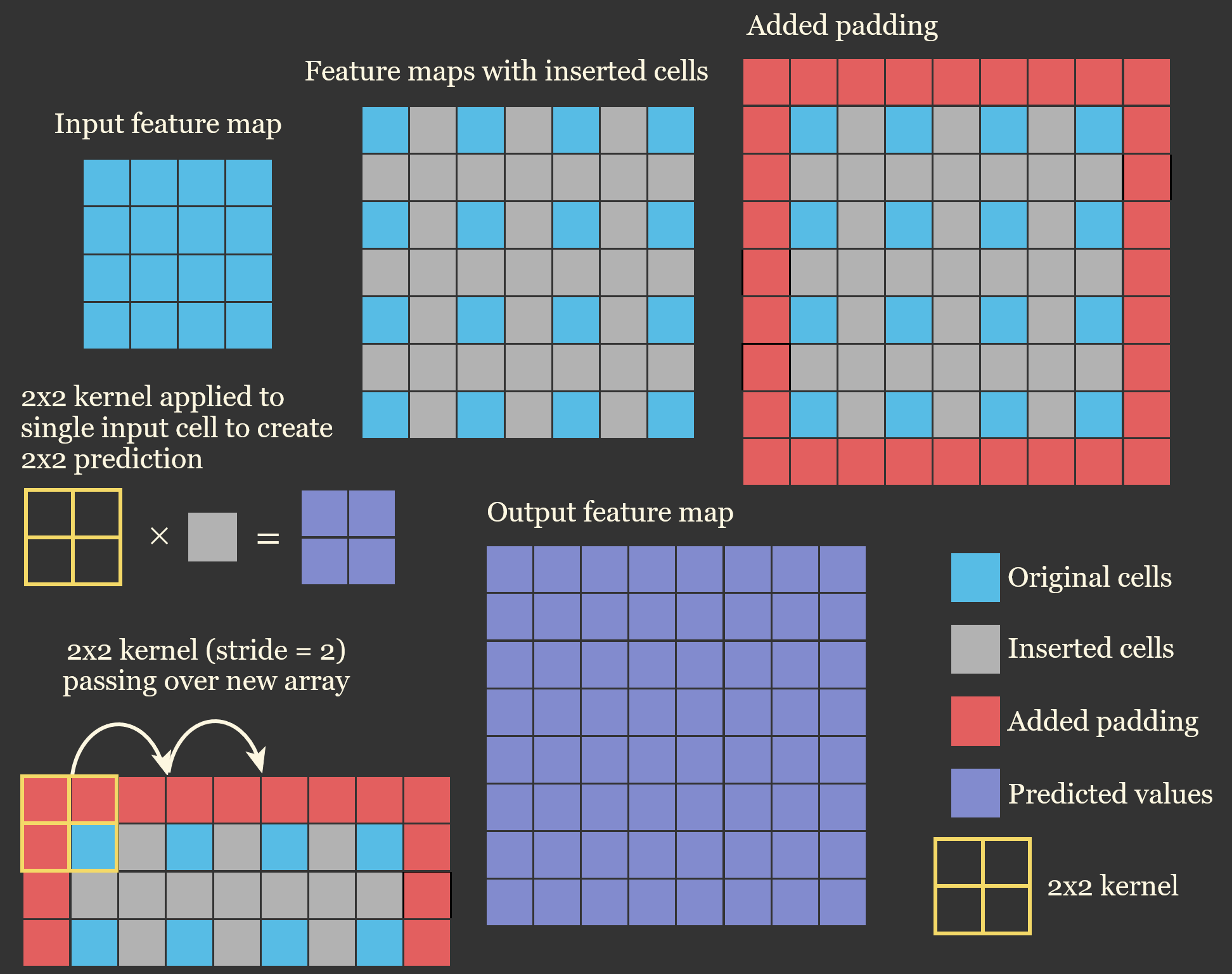
As demonstrated using the code below, 2D transpose convolution with a kernel size of 2x2 and a stride of 2 converts a tensor of shape (1,1,9,9) to a shape of (1,1,18,18). Since weights are applied, it requires that both an input tensor and kernel be provided.
inT = torch.rand(1,1,9,9)
inT
tensor([[[[0.1870, 0.3736, 0.5318, 0.2646, 0.1567, 0.9953, 0.3286, 0.5445,
0.2582],
[0.0984, 0.6659, 0.6627, 0.8498, 0.8462, 0.0392, 0.7246, 0.0808,
0.7368],
[0.5401, 0.1437, 0.5401, 0.1519, 0.9730, 0.2074, 0.2972, 0.9720,
0.3678],
[1.0000, 0.2718, 0.0334, 0.7357, 0.5191, 0.3519, 0.3619, 0.1834,
0.3035],
[0.1047, 0.6689, 0.9824, 0.1520, 0.8673, 0.4382, 0.4728, 0.6926,
0.1565],
[0.3443, 0.7002, 0.3636, 0.2952, 0.5435, 0.8644, 0.9594, 0.1376,
0.3396],
[0.9585, 0.6877, 0.1384, 0.1654, 0.1166, 0.9689, 0.9617, 0.2264,
0.3747],
[0.9920, 0.4840, 0.1309, 0.5416, 0.3788, 0.0256, 0.1416, 0.2536,
0.9396],
[0.9059, 0.0787, 0.3381, 0.2500, 0.9078, 0.1527, 0.1816, 0.2124,
0.1403]]]])inW = torch.rand(1,1,2,2)
inWtensor([[[[0.7886, 0.5281],
[0.8325, 0.8577]]]])outT = F.conv_transpose2d(inT, inW, stride=2, padding=0)
outT.shapetorch.Size([1, 1, 18, 18])In the example below, I have created a new 2x2 kernel in which the bottom-right value is 1 and all other values are 0. When applying this kernel, you can see that it results in expanding the array by adding rows and columns of zeros. When the weights are not set to zero, these added rows and columns can hold non-zero values. The kernel weights are trainable, resulting in the model learning how to upsample the image as opposed to simply applying an interpolation algorithm.
In the next example, I have performed 2D transpose convolution using a 2x2 kernel in which all weights are set to 1. This result is equivalent to performing nearest neighbor interpolation.
In later modules, you will see examples of deconvolution in action in the context of semantic segmentation. I will primarily rely on 2D transpose convolution as opposed to upsampling.
inW = torch.tensor([[[[0., 0.], [0., 1.]]]])outT = F.conv_transpose2d(inT, inW, stride=2, padding=0)
outT.shape
outTtensor([[[[0.0000, 0.0000, 0.0000, 0.0000, 0.0000, 0.0000, 0.0000, 0.0000,
0.0000, 0.0000, 0.0000, 0.0000, 0.0000, 0.0000, 0.0000, 0.0000,
0.0000, 0.0000],
[0.0000, 0.1870, 0.0000, 0.3736, 0.0000, 0.5318, 0.0000, 0.2646,
0.0000, 0.1567, 0.0000, 0.9953, 0.0000, 0.3286, 0.0000, 0.5445,
0.0000, 0.2582],
[0.0000, 0.0000, 0.0000, 0.0000, 0.0000, 0.0000, 0.0000, 0.0000,
0.0000, 0.0000, 0.0000, 0.0000, 0.0000, 0.0000, 0.0000, 0.0000,
0.0000, 0.0000],
[0.0000, 0.0984, 0.0000, 0.6659, 0.0000, 0.6627, 0.0000, 0.8498,
0.0000, 0.8462, 0.0000, 0.0392, 0.0000, 0.7246, 0.0000, 0.0808,
0.0000, 0.7368],
[0.0000, 0.0000, 0.0000, 0.0000, 0.0000, 0.0000, 0.0000, 0.0000,
0.0000, 0.0000, 0.0000, 0.0000, 0.0000, 0.0000, 0.0000, 0.0000,
0.0000, 0.0000],
[0.0000, 0.5401, 0.0000, 0.1437, 0.0000, 0.5401, 0.0000, 0.1519,
0.0000, 0.9730, 0.0000, 0.2074, 0.0000, 0.2972, 0.0000, 0.9720,
0.0000, 0.3678],
[0.0000, 0.0000, 0.0000, 0.0000, 0.0000, 0.0000, 0.0000, 0.0000,
0.0000, 0.0000, 0.0000, 0.0000, 0.0000, 0.0000, 0.0000, 0.0000,
0.0000, 0.0000],
[0.0000, 1.0000, 0.0000, 0.2718, 0.0000, 0.0334, 0.0000, 0.7357,
0.0000, 0.5191, 0.0000, 0.3519, 0.0000, 0.3619, 0.0000, 0.1834,
0.0000, 0.3035],
[0.0000, 0.0000, 0.0000, 0.0000, 0.0000, 0.0000, 0.0000, 0.0000,
0.0000, 0.0000, 0.0000, 0.0000, 0.0000, 0.0000, 0.0000, 0.0000,
0.0000, 0.0000],
[0.0000, 0.1047, 0.0000, 0.6689, 0.0000, 0.9824, 0.0000, 0.1520,
0.0000, 0.8673, 0.0000, 0.4382, 0.0000, 0.4728, 0.0000, 0.6926,
0.0000, 0.1565],
[0.0000, 0.0000, 0.0000, 0.0000, 0.0000, 0.0000, 0.0000, 0.0000,
0.0000, 0.0000, 0.0000, 0.0000, 0.0000, 0.0000, 0.0000, 0.0000,
0.0000, 0.0000],
[0.0000, 0.3443, 0.0000, 0.7002, 0.0000, 0.3636, 0.0000, 0.2952,
0.0000, 0.5435, 0.0000, 0.8644, 0.0000, 0.9594, 0.0000, 0.1376,
0.0000, 0.3396],
[0.0000, 0.0000, 0.0000, 0.0000, 0.0000, 0.0000, 0.0000, 0.0000,
0.0000, 0.0000, 0.0000, 0.0000, 0.0000, 0.0000, 0.0000, 0.0000,
0.0000, 0.0000],
[0.0000, 0.9585, 0.0000, 0.6877, 0.0000, 0.1384, 0.0000, 0.1654,
0.0000, 0.1166, 0.0000, 0.9689, 0.0000, 0.9617, 0.0000, 0.2264,
0.0000, 0.3747],
[0.0000, 0.0000, 0.0000, 0.0000, 0.0000, 0.0000, 0.0000, 0.0000,
0.0000, 0.0000, 0.0000, 0.0000, 0.0000, 0.0000, 0.0000, 0.0000,
0.0000, 0.0000],
[0.0000, 0.9920, 0.0000, 0.4840, 0.0000, 0.1309, 0.0000, 0.5416,
0.0000, 0.3788, 0.0000, 0.0256, 0.0000, 0.1416, 0.0000, 0.2536,
0.0000, 0.9396],
[0.0000, 0.0000, 0.0000, 0.0000, 0.0000, 0.0000, 0.0000, 0.0000,
0.0000, 0.0000, 0.0000, 0.0000, 0.0000, 0.0000, 0.0000, 0.0000,
0.0000, 0.0000],
[0.0000, 0.9059, 0.0000, 0.0787, 0.0000, 0.3381, 0.0000, 0.2500,
0.0000, 0.9078, 0.0000, 0.1527, 0.0000, 0.1816, 0.0000, 0.2124,
0.0000, 0.1403]]]])inW = torch.tensor([[[[1., 1.], [1., 1.]]]])
outT = F.conv_transpose2d(inT, inW, stride=2, padding=0)
outT.shape
outTtensor([[[[0.1870, 0.1870, 0.3736, 0.3736, 0.5318, 0.5318, 0.2646, 0.2646,
0.1567, 0.1567, 0.9953, 0.9953, 0.3286, 0.3286, 0.5445, 0.5445,
0.2582, 0.2582],
[0.1870, 0.1870, 0.3736, 0.3736, 0.5318, 0.5318, 0.2646, 0.2646,
0.1567, 0.1567, 0.9953, 0.9953, 0.3286, 0.3286, 0.5445, 0.5445,
0.2582, 0.2582],
[0.0984, 0.0984, 0.6659, 0.6659, 0.6627, 0.6627, 0.8498, 0.8498,
0.8462, 0.8462, 0.0392, 0.0392, 0.7246, 0.7246, 0.0808, 0.0808,
0.7368, 0.7368],
[0.0984, 0.0984, 0.6659, 0.6659, 0.6627, 0.6627, 0.8498, 0.8498,
0.8462, 0.8462, 0.0392, 0.0392, 0.7246, 0.7246, 0.0808, 0.0808,
0.7368, 0.7368],
[0.5401, 0.5401, 0.1437, 0.1437, 0.5401, 0.5401, 0.1519, 0.1519,
0.9730, 0.9730, 0.2074, 0.2074, 0.2972, 0.2972, 0.9720, 0.9720,
0.3678, 0.3678],
[0.5401, 0.5401, 0.1437, 0.1437, 0.5401, 0.5401, 0.1519, 0.1519,
0.9730, 0.9730, 0.2074, 0.2074, 0.2972, 0.2972, 0.9720, 0.9720,
0.3678, 0.3678],
[1.0000, 1.0000, 0.2718, 0.2718, 0.0334, 0.0334, 0.7357, 0.7357,
0.5191, 0.5191, 0.3519, 0.3519, 0.3619, 0.3619, 0.1834, 0.1834,
0.3035, 0.3035],
[1.0000, 1.0000, 0.2718, 0.2718, 0.0334, 0.0334, 0.7357, 0.7357,
0.5191, 0.5191, 0.3519, 0.3519, 0.3619, 0.3619, 0.1834, 0.1834,
0.3035, 0.3035],
[0.1047, 0.1047, 0.6689, 0.6689, 0.9824, 0.9824, 0.1520, 0.1520,
0.8673, 0.8673, 0.4382, 0.4382, 0.4728, 0.4728, 0.6926, 0.6926,
0.1565, 0.1565],
[0.1047, 0.1047, 0.6689, 0.6689, 0.9824, 0.9824, 0.1520, 0.1520,
0.8673, 0.8673, 0.4382, 0.4382, 0.4728, 0.4728, 0.6926, 0.6926,
0.1565, 0.1565],
[0.3443, 0.3443, 0.7002, 0.7002, 0.3636, 0.3636, 0.2952, 0.2952,
0.5435, 0.5435, 0.8644, 0.8644, 0.9594, 0.9594, 0.1376, 0.1376,
0.3396, 0.3396],
[0.3443, 0.3443, 0.7002, 0.7002, 0.3636, 0.3636, 0.2952, 0.2952,
0.5435, 0.5435, 0.8644, 0.8644, 0.9594, 0.9594, 0.1376, 0.1376,
0.3396, 0.3396],
[0.9585, 0.9585, 0.6877, 0.6877, 0.1384, 0.1384, 0.1654, 0.1654,
0.1166, 0.1166, 0.9689, 0.9689, 0.9617, 0.9617, 0.2264, 0.2264,
0.3747, 0.3747],
[0.9585, 0.9585, 0.6877, 0.6877, 0.1384, 0.1384, 0.1654, 0.1654,
0.1166, 0.1166, 0.9689, 0.9689, 0.9617, 0.9617, 0.2264, 0.2264,
0.3747, 0.3747],
[0.9920, 0.9920, 0.4840, 0.4840, 0.1309, 0.1309, 0.5416, 0.5416,
0.3788, 0.3788, 0.0256, 0.0256, 0.1416, 0.1416, 0.2536, 0.2536,
0.9396, 0.9396],
[0.9920, 0.9920, 0.4840, 0.4840, 0.1309, 0.1309, 0.5416, 0.5416,
0.3788, 0.3788, 0.0256, 0.0256, 0.1416, 0.1416, 0.2536, 0.2536,
0.9396, 0.9396],
[0.9059, 0.9059, 0.0787, 0.0787, 0.3381, 0.3381, 0.2500, 0.2500,
0.9078, 0.9078, 0.1527, 0.1527, 0.1816, 0.1816, 0.2124, 0.2124,
0.1403, 0.1403],
[0.9059, 0.9059, 0.0787, 0.0787, 0.3381, 0.3381, 0.2500, 0.2500,
0.9078, 0.9078, 0.1527, 0.1527, 0.1816, 0.1816, 0.2124, 0.2124,
0.1403, 0.1403]]]])9.6 Concluding Remarks
Now that we have investigated the common layers used to build CNNs, we will move on to actually creating them. In the next section relating to CNNs for scene labeling, we will primarily make use of nn.Conv2d() and nn.MaxPool2d() along with layers we have investigated while implementing fully connected neural networks: nn.Linear(), nn.ReLU(), and nn.BatchNorm2d(). In later modules you will see applications of nn.ConvTranspose2d() for upsampling.
9.7 Questions
- Explain the purposes of the stride and padding parameters when applying 2D convolution. What padding is required to maintain the height and width of the input when using a 3x3 kernel and a stride of 1?
- An input tensor has a shape of (1, 1, 9, 9). What will be the shape of the output if three 3x3 kernels are applied using a stride of 1 and a padding of 0?
- Explain how max pooling with a 2x2 window and a stride of 2 changes the size of a tensor. How does average pooling differ from max pooling?
- Why must activation functions be included in CNN architectures? Explain how the ReLU and leaky ReLU activation functions differ.
- Explain the difference between the sigmoid and softmax activation functions and when each is used.
- For each of the following PyTorch loss functions, state whether it expects raw logits or probabilities:
nn.CrossEntropyLoss(),nn.NLLLoss(),nn.BCELoss(), andnn.BCEWithLogitsLoss(). - Explain the difference between increasing the spatial dimensions of a tensor using interpolation-based upsampling and using 2D transpose convolution. Which method has trainable parameters?
- Why are upsampling operations required for semantic segmentation but not for scene labeling? A tensor with a shape of (1, 16, 32, 32) is passed through a 2D transpose convolution layer with a 2x2 kernel, a stride of 2, and 8 output channels. What will be the shape of the output?