import warnings
import numpy as np
import pandas as pd
import matplotlib.pyplot as plt
import rasterio as rio
from rasterio import features
from rasterio.transform import rowcol
from rasterio.windows import Window
import geopandas as gpd
from shapely.geometry import shape
from scipy import ndimage

import torch
import torch.nn.functional as F
from torch.utils.data import Dataset, DataLoader
import lightning as L
from lightning.pytorch.loggers import CSVLogger
from sam2.sam2_image_predictor import SAM2ImagePredictor
from sam2.automatic_mask_generator import SAM2AutomaticMaskGenerator

from huggingface_hub.utils import logging as hfLogging

warnings.filterwarnings("ignore", module="sam2")
hfLogging.set_verbosity_error()   # hide Hugging Face Hub download notices
device = torch.device("cuda" if torch.cuda.is_available() else "cpu")28 Foundation Models and Segment Anything
28.1 Introduction
A foundation model is a large model trained on a very large and diverse dataset, generally using self-supervised or weakly supervised learning, that can be adapted to many downstream tasks. Large language models are the most familiar example. In computer vision, foundation models include CLIP, which relates images and text; DINOv2, which provides general-purpose image features learned through self-supervision; and the Segment Anything Model (SAM), which segments objects in images given simple prompts. There are also a growing number of geospatial foundation models, which are pre-trained on large archives of satellite or aerial imagery. Examples include Prithvi, developed by NASA and IBM using Harmonized Landsat and Sentinel-2 data; SatMAE; and Clay. Many of these are pre-trained using masked autoencoding, the approach explored in Chapter 27.
Foundation models share several characteristics:
- They are trained on far more data than is available for most individual applications, often hundreds of millions of images.
- They are large, with hundreds of millions or billions of parameters, and are generally based on transformer architectures (Chapter 25), which scale well with data and model size.
- They can be applied to new problems with little or no task-specific training, either directly (zero-shot) or after fine-tuning with a small labeled dataset (few-shot).
In this chapter, I focus on applying SAM 2 to geospatial imagery using a practical mapping problem: extracting poultry houses from leaf-off aerial imagery. Poultry production is concentrated in parts of West Virginia, especially the South Branch Potomac River valley in the eastern part of the state. Poultry litter and runoff from poultry operations can be a source of nutrient and bacterial pollution to streams, which ultimately drain to the Chesapeake Bay. Mapping the locations and footprints of poultry houses is therefore useful for assessing and managing these pollution sources. Poultry houses are well suited to SAM: they are generally large, often have bright roofs with distinct boundaries, and are long, narrow rectangles. However, they are also commonly arranged side-by-side, so that the separation of adjacent houses is an important part of the problem.
I demonstrate how to segment poultry houses using point, box, and mask prompts without any training, how to automatically generate masks for an entire image and filter them to the features of interest, and how to fine-tune SAM 2’s mask decoder using fewer than 10 labeled poultry houses. All of the models are assessed using poultry houses that were not used for fine-tuning. I also discuss how to process large images, how SAM can be combined with the models trained in earlier chapters, and the limitations of applying SAM to geospatial data.
28.2 The Segment Anything Model
The original SAM (Kirillov et al., 2023) was trained on SA-1B, a dataset of 11 million images and more than 1 billion masks, which was generated in part by using early versions of the model to help annotators label images. SAM has three components:
- Image encoder: a large Vision Transformer, pre-trained as a masked autoencoder, that computes an embedding of the image. This is the most computationally expensive component, but it is run only once per image.
- Prompt encoder: converts prompts, such as points (labeled as foreground or background), boxes, or rough masks, into embeddings.
- Mask decoder: a lightweight transformer that combines the image and prompt embeddings to predict masks. Since a single prompt can be ambiguous (e.g., a point on a roof could indicate the roof, the building, or the entire block), the decoder can return several candidate masks along with a predicted IoU score for each, which estimates the quality of the mask.
Kirillov, A., Mintun, E., Ravi, N., Mao, H., Rolland, C., Gustafson, L., Xiao, T., Whitehead, S., Berg, A.C., Lo, W.Y. and Dollár, P., 2023. “Segment anything.” In Proceedings of the IEEE/CVF International Conference on Computer Vision (pp. 4015-4026).
Because the image embedding is computed once and the decoder is fast, many prompts can be applied to the same image interactively. SAM 2 (Ravi et al., 2024) extends SAM to video by adding a memory mechanism that stores information about the objects segmented in previous frames, allowing objects to be tracked through a sequence. It uses a hierarchical transformer image encoder, called Hiera, which is faster than SAM’s encoder and produces multi-scale features, and it was trained on a large video dataset, SA-V, in addition to SA-1B. For single images, SAM 2 is both faster and more accurate than SAM. The video capabilities may also be relevant to time series of geospatial imagery. Meta has continued to release newer versions of SAM, so check the current options when starting a new project.
Ravi, N., Gabeur, V., Hu, Y.T., Hu, R., Ryali, C., Ma, T., Khedr, H., Rädle, R., Rolland, C., Gustafson, L. and Mintun, E., 2024. “SAM 2: Segment anything in images and videos.” arXiv preprint arXiv:2408.00714.
An important characteristic of SAM is that it is class-agnostic: it segments objects or regions but does not assign them to classes. It can delineate a building, a field, or a pond, but it does not know what they are. As we will see, this means that SAM is generally combined with prompts that identify the features of interest or with another method that identifies which of its outputs represent the features of interest.
28.3 Setup
SAM 2 is installed from its GitHub repository following the instructions provided there (https://github.com/facebookresearch/sam2). Pre-trained checkpoints are available in several sizes (tiny, small, base plus, and large), which trade speed for accuracy, and they can be downloaded automatically from Hugging Face using the from_pretrained() methods demonstrated below. A CUDA-enabled GPU is strongly recommended. SAM 2 is generally run using bfloat16 mixed precision and inference mode, which disables gradient calculations. If SAM 2’s optional CUDA extension is not compiled during installation, it warns that it is skipping a post-processing step that fills small holes in the masks. This can be safely ignored, so I suppress this warning.
28.4 Poultry House Data
28.4.1 Imagery and Reference Polygons
The imagery was collected in 2003 for the West Virginia Statewide Addressing and Mapping Board (SAMB) during leaf-off conditions. It has three bands (red, green, and blue) with 8-bit radiometric resolution and a spatial resolution of 2 feet (0.6096 m). The subset used here covers part of the South Branch Potomac River valley near Moorefield in Hardy County, West Virginia. The poultry houses in this extent were digitized from the imagery by the author and are provided as reference polygons in a shapefile. The data are provided with the text in the data/files/forSAM folder. Both datasets use the NAD83 UTM Zone 17N projection. Poultry houses are typically 13 to 23 m wide and up to 190 m long, or roughly 20 to 40 pixels wide and up to 300 pixels long in this imagery.
folder = "data/files/forSAM/"
imgPath = folder + "sambImagery.tif"

with rio.open(imgPath) as src:
    print(src.count, src.dtypes, src.res, src.width, src.height, src.crs)
3 ('uint8', 'uint8', 'uint8') (0.6096009999999988, 0.6096010000000154) 19244 24146 EPSG:26917houses = gpd.read_file(folder + "poultryHouses.shp")[["geometry"]]
houses["houseID"] = np.arange(len(houses))
print(len(houses))63print(houses.area.describe())count 63.000000
mean 1753.533340
std 491.533548
min 427.272457
25% 1401.929241
50% 1860.969651
75% 2074.206246
max 2937.104191
dtype: float6428.4.2 Training and Test Houses
I will fine-tune SAM using only eight poultry houses and assess all of the models using houses that were not used for fine-tuning. Since poultry houses on the same farm are generally identical in construction and age and are adjacent to each other, using one house on a farm for training and its neighbor for testing would overestimate performance. So, I first group the houses into farms by buffering each house by 75 m and dissolving the overlapping buffers. Each farm is a separate polygon, and each house is assigned the ID of the farm it falls within using a spatial join.
I then randomly select eight farms and one house from each of these farms for training. All houses on the remaining farms are used for testing. The other houses on the training farms are not used, since they are not independent of the training houses. This results in 8 training houses, 46 test houses from 16 farms, and 9 unused houses. The training houses are spread across 8 farms, which provides more variability in roof appearance, house size, and surroundings than using several houses from the same farm.
farmGeoms = houses.buffer(75).union_all()
farms = gpd.GeoDataFrame({"farmID": np.arange(len(farmGeoms.geoms))},
                         geometry=list(farmGeoms.geoms), crs=houses.crs)
houses = gpd.sjoin(houses, farms, predicate="within").drop(columns="index_right")
houses = houses.sort_values("houseID")

rng = np.random.default_rng(42)
trainFarms = np.sort(rng.choice(farms["farmID"], size=8, replace=False))
trainIDs = [int(rng.choice(houses.loc[houses["farmID"] == f, "houseID"])) for f in trainFarms]

houses["split"] = "test"
houses.loc[houses["farmID"].isin(trainFarms), "split"] = "unused"
houses.loc[houses["houseID"].isin(trainIDs), "split"] = "train"
testIDs = houses.loc[houses["split"] == "test", "houseID"].tolist()

print(len(farms))24print(houses["split"].value_counts())split
test 46
unused 9
train 8
Name: count, dtype: int64The map below shows the locations of the poultry houses over the imagery. To display the large image quickly, I read it at 1/32 of its full resolution by specifying an out_shape, which allows Rasterio to use the image’s overviews (pyramids).
with rio.open(imgPath) as src:
    ovr = src.read(out_shape=(3, src.height // 32, src.width // 32))
    extent = (src.bounds.left, src.bounds.right, src.bounds.bottom, src.bounds.top)

fig, ax = plt.subplots(figsize=(8, 10))
ax.imshow(np.transpose(ovr, (1, 2, 0)), extent=extent)
for split, color in {"train": "red", "test": "yellow", "unused": "cyan"}.items():
    houses[houses["split"] == split].centroid.plot(ax=ax, color=color, markersize=15, label=split)
ax.legend()
ax.set_axis_off()
plt.show()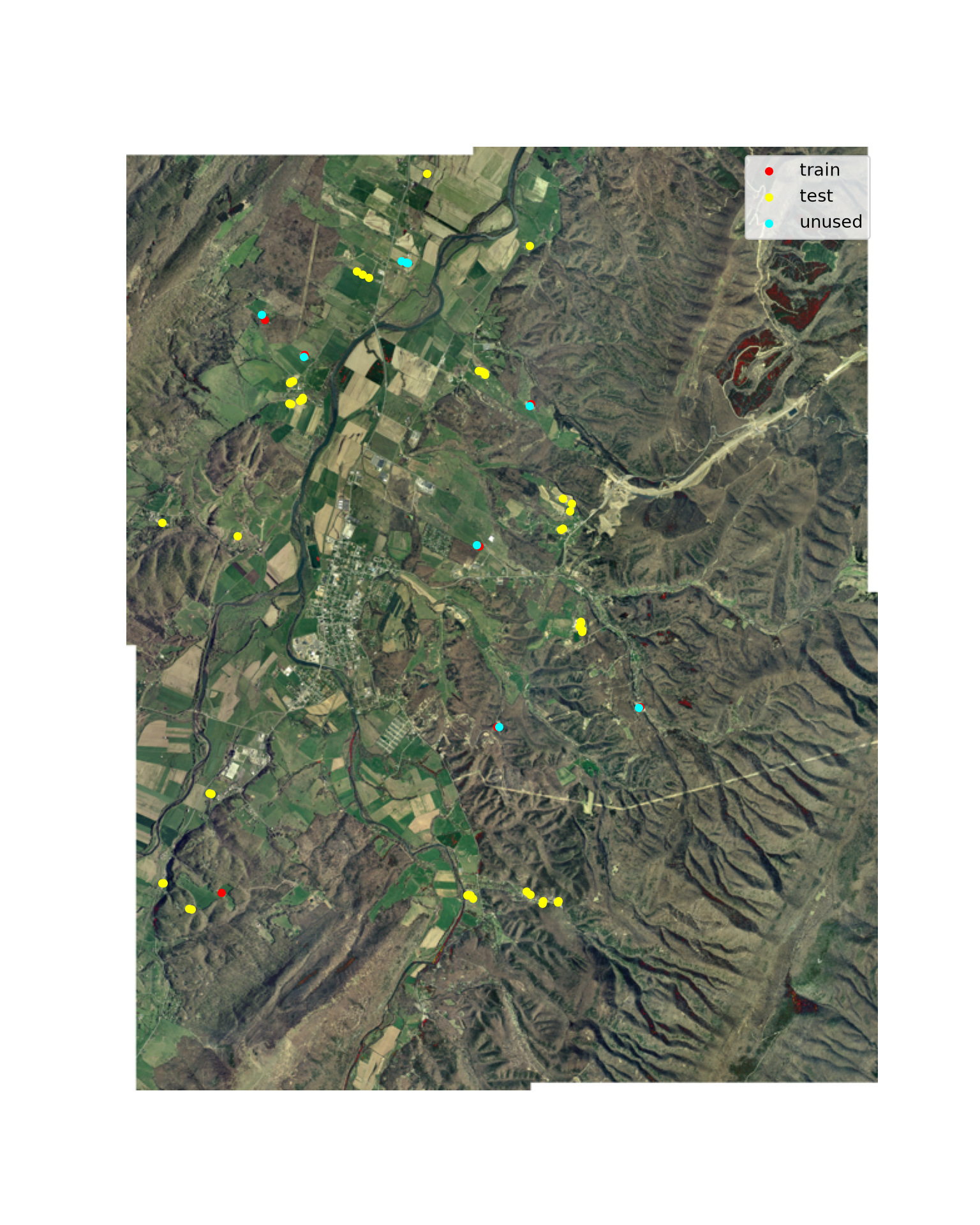
28.4.3 Image Chips
SAM 2 resizes each input image to 1024x1024 pixels, so it should be provided with image chips as opposed to the entire image. I extract a 512x512 pixel (312x312 m) chip centered on each poultry house, which is large enough to contain the largest houses along with their surroundings. Since SAM upsamples the 512x512 chips to 1024x1024, small details, such as the gaps between adjacent houses, are enlarged. The getChip() function reads the chip using a Rasterio window, obtains the chip’s affine transform, which is needed to convert between pixel and map coordinates, and rasterizes the house’s polygon to create a binary reference mask. Note that the mask only includes the house the chip is centered on, not its neighbors, since SAM is used to segment one object at a time.
The SAMB imagery is already 8-bit, three-band RGB, which is the format SAM expects, so no conversion is needed. Imagery with more than three bands or a greater bit depth must be converted to three 8-bit bands first, for example, by selecting bands and applying a percentile stretch. Since SAM was trained on natural color photographs, it may perform best with natural color imagery, although false color composites may better differentiate some features.
CHIP = 512

def getChip(src, geom, size=CHIP):
    cx, cy = geom.centroid.coords[0]
    row, col = src.index(cx, cy)
    win = Window(col - size // 2, row - size // 2, size, size)
    img = np.transpose(src.read([1, 2, 3], window=win), (1, 2, 0))   # (H, W, 3)
    transform = src.window_transform(win)
    mask = features.rasterize([(geom, 1)], out_shape=(size, size), transform=transform, dtype="uint8")
    return img, mask, transform

chips = {}
with rio.open(imgPath) as src:
    for hid, geom in zip(houses["houseID"], houses.geometry):
        chips[hid] = getChip(src, geom)
The training houses are shown below with their reference polygons outlined in red. Note the variability in roof brightness, house length, and surroundings, as well as the presence of adjacent houses.
fig, axs = plt.subplots(2, 4, figsize=(16, 8))
for ax, hid in zip(axs.flat, trainIDs):
    img, mask, _ = chips[hid]
    ax.imshow(img)
    ax.contour(mask, levels=[0.5], colors="red", linewidths=1)
    ax.set_title(f"House {hid}")
    ax.axis("off")
plt.tight_layout()
plt.show()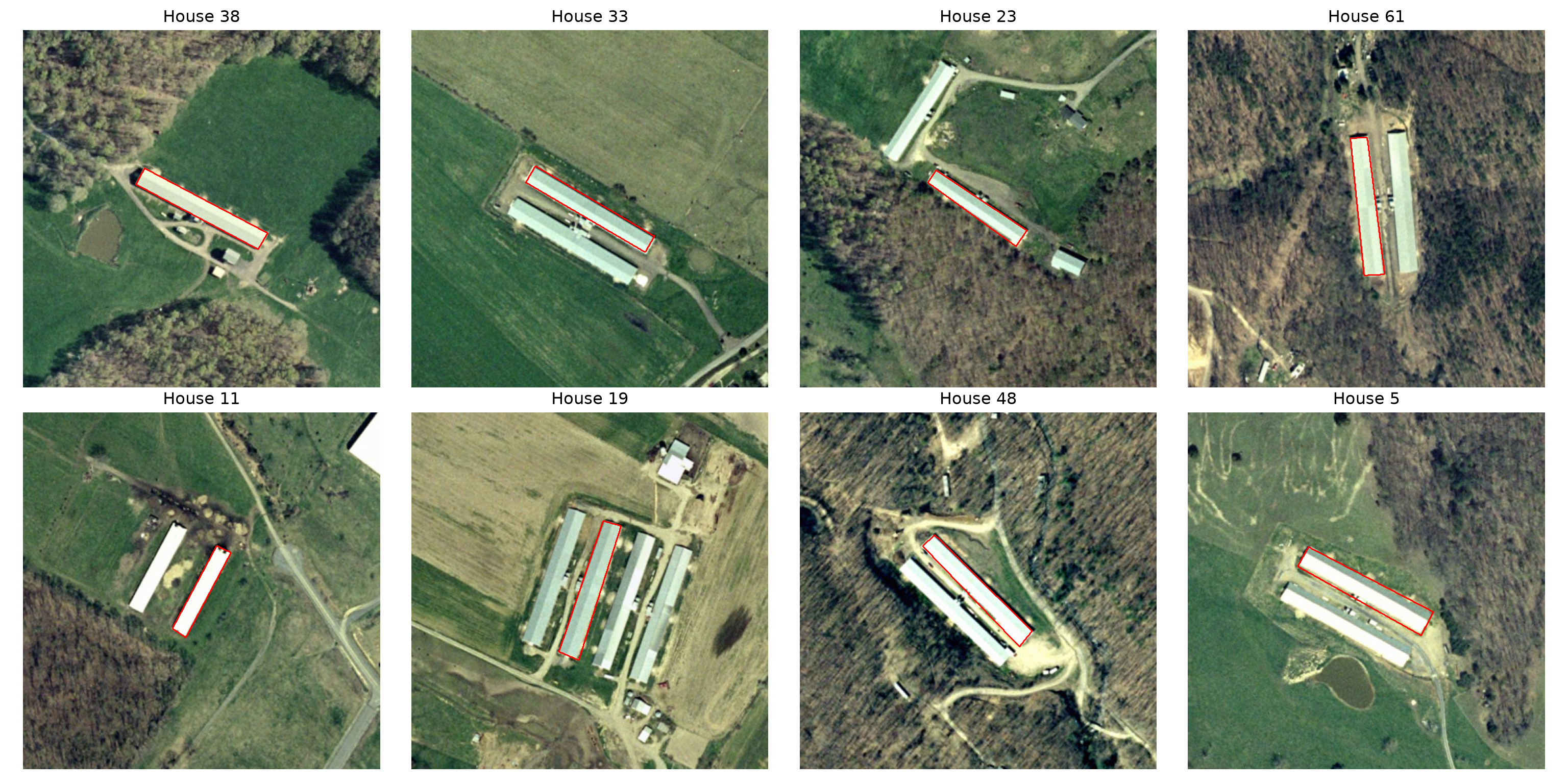
28.5 Zero-Shot Prompted Segmentation
28.5.1 Helper Functions
I next define several helper functions. maskToBox() returns the bounding box of a mask in pixel coordinates as (xmin, ymin, xmax, ymax). pointPrompt() converts a point inside a polygon to pixel coordinates using the Rasterio rowcol() function and the chip’s transform. I use the representative_point() method as opposed to the centroid since it is guaranteed to fall within the polygon. axisPoints() returns points at 25% and 75% of the distance along the long axis of the polygon’s minimum rotated rectangle, which provides two points that are spread along the house. SAM expects points as (x, y), or (column, row), coordinates. iou() calculates the intersection-over-union between a predicted and reference mask, and showMask() plots a predicted mask in red over the image along with the reference outline in cyan and, optionally, the prompts. The zoom argument crops the display to the house plus a buffer, in pixels.
In practice, prompts would come from an existing data source, such as point locations of poultry operations from a permit database or approximate boxes from an object detector. Here, I derive them from the reference polygons to simulate such data.
def maskToBox(mask):
    rows, cols = np.where(mask > 0)
    return np.array([cols.min(), rows.min(), cols.max(), rows.max()])

def pointPrompt(geom, transform):
    pt = geom.representative_point()
    row, col = rowcol(transform, pt.x, pt.y)
    return np.array([[col, row]])

def axisPoints(geom, transform, fracs=(0.25, 0.75)):
    c = np.array(geom.minimum_rotated_rectangle.exterior.coords)[:4]
    if np.linalg.norm(c[1] - c[0]) < np.linalg.norm(c[2] - c[1]):
        a, b = (c[0] + c[1]) / 2, (c[2] + c[3]) / 2   # midpoints of the short sides
    else:
        a, b = (c[1] + c[2]) / 2, (c[3] + c[0]) / 2
    pts = [a + f * (b - a) for f in fracs]
    return np.array([rowcol(transform, x, y)[::-1] for x, y in pts])

def iou(pred, ref):
    pred, ref = pred > 0, ref > 0
    return (pred & ref).sum() / (pred | ref).sum()

def showMask(ax, img, pred, ref, title="", points=None, box=None, zoom=None):
    ax.imshow(img)
    ax.imshow(np.ma.masked_where(pred == 0, pred), alpha=0.5, cmap="autumn")
    ax.contour(ref, levels=[0.5], colors="cyan", linewidths=1)
    if points is not None:
        ax.scatter(points[:, 0], points[:, 1], c="yellow", s=40, edgecolors="black")
    if box is not None:
        ax.add_patch(plt.Rectangle((box[0], box[1]), box[2] - box[0], box[3] - box[1],
                                   fill=False, edgecolor="yellow", linewidth=1.5))
    if zoom is not None:   # crop the display to the reference mask plus a buffer of zoom pixels
        x0, y0, x1, y1 = maskToBox(ref)
        ax.set_xlim(x0 - zoom, x1 + zoom)
        ax.set_ylim(y1 + zoom, y0 - zoom)
    ax.set_title(title)
    ax.axis("off")
28.5.2 Point Prompts
The SAM2ImagePredictor class provides prompted segmentation for single images. I load the large SAM 2.1 model, which has 224 million parameters. The set_image() method computes and stores the image embedding, and the predict() method generates masks for a set of prompts. Point prompts are provided as pixel coordinates along with labels: 1 for a point on the object (foreground) and 0 for a point that is not on the object (background). With multimask_output=True, three candidate masks are returned along with their predicted IoU scores.
The example below uses a single point on a test house whose roof consists of two sections with different brightness. The three candidate masks represent different interpretations of the prompt. Generally, the mask with the highest predicted IoU score is kept. However, the predicted score does not always identify the mask that best matches the feature of interest, since SAM has no way of knowing whether we are interested in one roof section or the entire house.
predictor = SAM2ImagePredictor.from_pretrained("facebook/sam2.1-hiera-large", device=device)

hid = 49
img, mask, tr = chips[hid]
pt = pointPrompt(houses.geometry[hid], tr)

with torch.inference_mode(), torch.autocast("cuda", dtype=torch.bfloat16):
    predictor.set_image(img)
    masks, scores, logits = predictor.predict(point_coords=pt, point_labels=np.array([1]),
                                              multimask_output=True)
print(masks.shape, scores)
(3, 512, 512) [0.734375 0.515625 0.6640625]fig, axs = plt.subplots(1, 3, figsize=(15, 5))
for i, ax in enumerate(axs):
showMask(ax, img, masks[i], mask, f"Score: {scores[i]:.3f}, IoU: {iou(masks[i], mask):.3f}", points=pt,
zoom=60)
plt.tight_layout()
plt.show()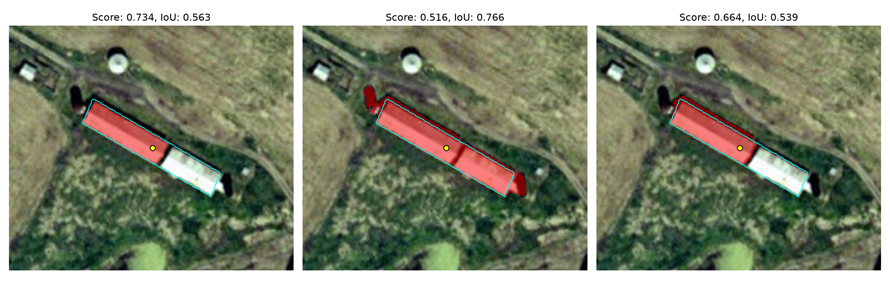
Additional foreground and background points can be added to refine a mask. For example, if the mask spills from a house onto an adjacent house, a background point on the adjacent house can be added. Below, I instead use two foreground points spread along the long axis of the house, which makes the prompt less ambiguous. When several points unambiguously identify an object, multimask_output=False can be used to return a single mask.
pts = axisPoints(houses.geometry[hid], tr)
with torch.inference_mode(), torch.autocast("cuda", dtype=torch.bfloat16):
    masks, scores, _ = predictor.predict(point_coords=pts, point_labels=np.array([1, 1]),
                                         multimask_output=False)

fig, ax = plt.subplots(figsize=(6, 6))
showMask(ax, img, masks[0], mask, f"IoU: {iou(masks[0], mask):.3f}", points=pts, zoom=60)
plt.show()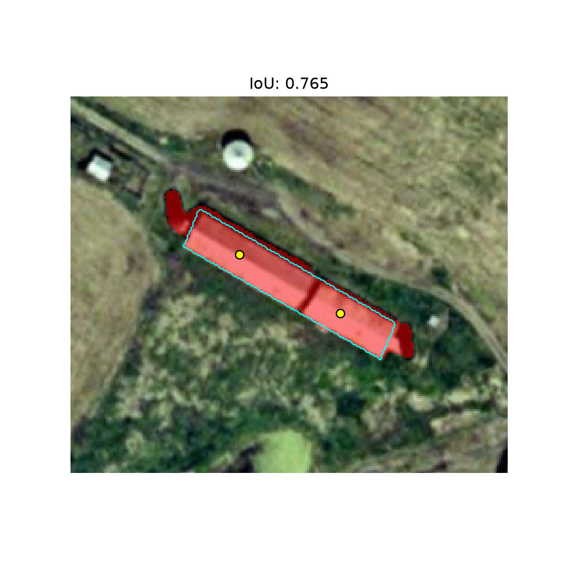
28.5.3 Box Prompts
A bounding box, given as (xmin, ymin, xmax, ymax) in pixel coordinates, is often a less ambiguous prompt than a single point. However, the box is aligned with the image’s rows and columns. For a house that is oriented diagonally, the box contains a large area outside of the house, which may include parts of adjacent houses, as in the example below. Multiple boxes can also be provided in a single call to segment several objects at once.
hid = 28
img, mask, tr = chips[hid]
box = maskToBox(mask)

with torch.inference_mode(), torch.autocast("cuda", dtype=torch.bfloat16):
    predictor.set_image(img)
    masks, scores, _ = predictor.predict(box=box, multimask_output=False)

fig, ax = plt.subplots(figsize=(6, 6))
showMask(ax, img, masks[0], mask, f"IoU: {iou(masks[0], mask):.3f}", box=box, zoom=100)
plt.show()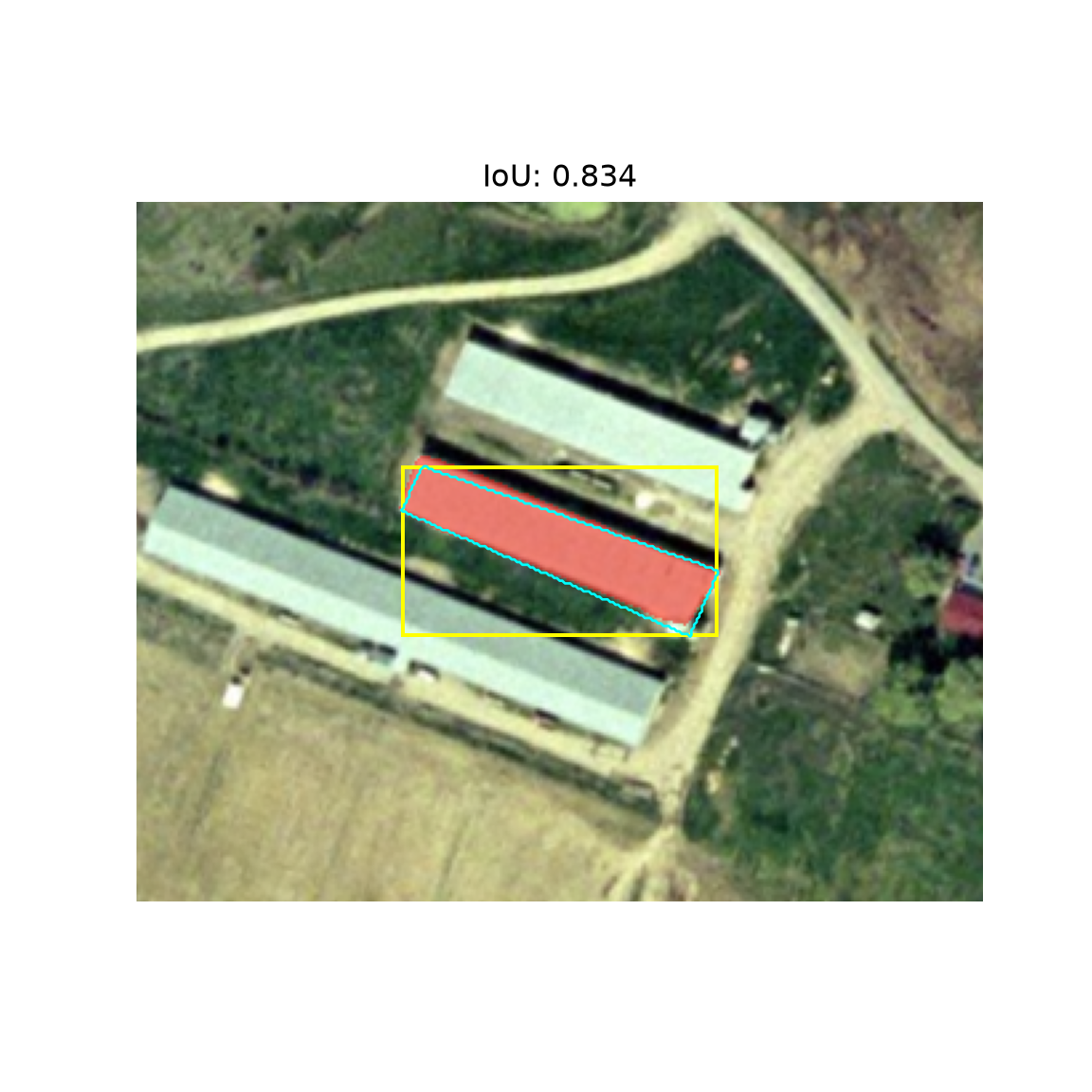
28.5.4 Mask Prompts
SAM also accepts a mask as a prompt using the mask_input argument. This is designed for iterative refinement: the low-resolution logits returned by one call to predict() are provided to the next call along with additional points. The mask prompt must therefore be provided as a 256x256 array of logits, which corresponds to SAM’s 1024x1024 input after downsampling by a factor of 4. The maskToLogits() function converts a binary mask to this format by resizing it to 256x256 and assigning large positive values to the object and large negative values to the background.
A geospatial application of mask prompts is refining existing polygons that are approximate, such as features digitized at a coarse scale or from older imagery. To simulate this, I create an approximate mask by dilating the reference mask by 8 pixels (~5 m) in all directions. I provide SAM with (1) the reference mask itself, (2) the approximate mask, and (3) the approximate mask along with its bounding box.
def maskToLogits(mask, value=10.0):
    t = torch.from_numpy(mask.astype("float32"))[None, None]
    t = F.interpolate(t, size=(256, 256), mode="bilinear", align_corners=False)
    return np.where(t[0].numpy() > 0.5, value, -value).astype("float32")   # (1, 256, 256)

def approxMask(mask, iterations=8):
    return ndimage.binary_dilation(mask, iterations=iterations).astype("uint8")

hid = 4
img, mask, tr = chips[hid]
approx = approxMask(mask)

with torch.inference_mode(), torch.autocast("cuda", dtype=torch.bfloat16):
    predictor.set_image(img)
    mRef, _, _ = predictor.predict(mask_input=maskToLogits(mask), multimask_output=False)
    mApprox, _, _ = predictor.predict(mask_input=maskToLogits(approx), multimask_output=False)
    mBoth, _, _ = predictor.predict(box=maskToBox(approx), mask_input=maskToLogits(approx),
                                    multimask_output=False)

fig, axs = plt.subplots(1, 4, figsize=(20, 5))
showMask(axs[0], img, approx, mask, f"Approximate mask, IoU: {iou(approx, mask):.3f}", zoom=40)
showMask(axs[1], img, mRef[0], mask, f"Reference mask prompt, IoU: {iou(mRef[0], mask):.3f}", zoom=40)
showMask(axs[2], img, mApprox[0], mask, f"Approximate mask prompt, IoU: {iou(mApprox[0], mask):.3f}", zoom=40)
showMask(axs[3], img, mBoth[0], mask, f"Box + approximate mask, IoU: {iou(mBoth[0], mask):.3f}", zoom=40)
plt.tight_layout()
plt.show()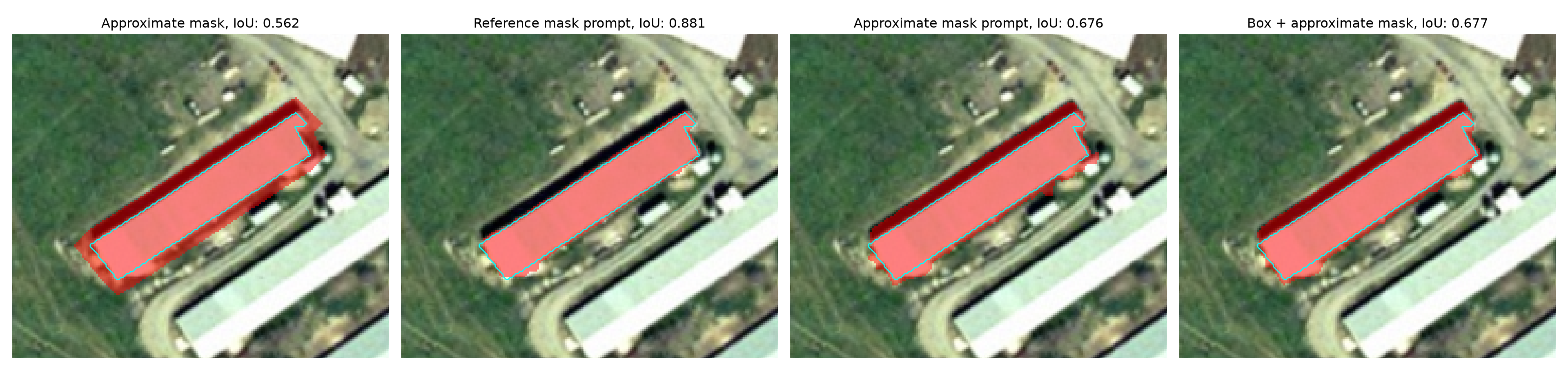
28.5.5 Assessing Prompts using the Test Houses
To compare the prompt types, I apply each of them to all of the test houses. The makePrompts() function returns a dictionary of keyword arguments for the predict() method for each prompt type, and assessPrompts() computes the image embedding once for each chip, applies each prompt type, keeps the candidate mask with the highest predicted IoU score, and calculates the IoU relative to the reference mask. It returns a DataFrame of IoU values and a dictionary of predicted masks. I also calculate the IoU of the approximate mask itself, which indicates how much SAM improves it.
def makePrompts(hid):
    img, mask, tr = chips[hid]
    geom = houses.geometry[hid]
    approx = approxMask(mask)
    return {"point": dict(point_coords=pointPrompt(geom, tr), point_labels=np.array([1]),
                          multimask_output=True),
            "twoPoints": dict(point_coords=axisPoints(geom, tr), point_labels=np.array([1, 1]),
                              multimask_output=False),
            "box": dict(box=maskToBox(mask), multimask_output=False),
            "refMask": dict(mask_input=maskToLogits(mask), multimask_output=False),
            "approxMask": dict(mask_input=maskToLogits(approx), multimask_output=False),
            "boxApproxMask": dict(box=maskToBox(approx), mask_input=maskToLogits(approx),
                                  multimask_output=False)}

def assessPrompts(predictor, ids, promptTypes):
    rows, preds = [], {}
    for hid in ids:
        img, mask, _ = chips[hid]
        prompts = makePrompts(hid)
        row, preds[hid] = {"houseID": hid}, {}
        with torch.inference_mode(), torch.autocast("cuda", dtype=torch.bfloat16):
            predictor.set_image(img)
            for p in promptTypes:
                masks, scores, _ = predictor.predict(**prompts[p])
                preds[hid][p] = masks[np.argmax(scores)]
                row[p] = iou(preds[hid][p], mask)
        rows.append(row)
    return pd.DataFrame(rows), preds

promptTypes = ["point", "twoPoints", "box", "refMask", "approxMask", "boxApproxMask"]
zsDF, zsPreds = assessPrompts(predictor, testIDs, promptTypes)
zsDF["approxInput"] = [iou(approxMask(chips[h][1]), chips[h][1]) for h in testIDs]
print(zsDF.drop(columns="houseID").describe().round(3).to_string())
point twoPoints box refMask approxMask boxApproxMask approxInput
count 46.000 46.000 46.000 46.000 46.000 46.000 46.000
mean 0.868 0.871 0.887 0.911 0.802 0.802 0.591
std 0.084 0.072 0.051 0.031 0.066 0.069 0.033
min 0.563 0.675 0.730 0.832 0.641 0.644 0.513
25% 0.853 0.833 0.871 0.893 0.747 0.747 0.572
50% 0.900 0.896 0.901 0.919 0.809 0.819 0.583
75% 0.914 0.918 0.918 0.929 0.848 0.858 0.607
max 0.955 0.956 0.958 0.966 0.911 0.918 0.671fig, ax = plt.subplots(figsize=(10, 5))
ax.boxplot([zsDF[p] for p in promptTypes], tick_labels=promptTypes)
ax.set_ylabel("IoU")
ax.set_title("Zero-shot IoU for test houses")
plt.show()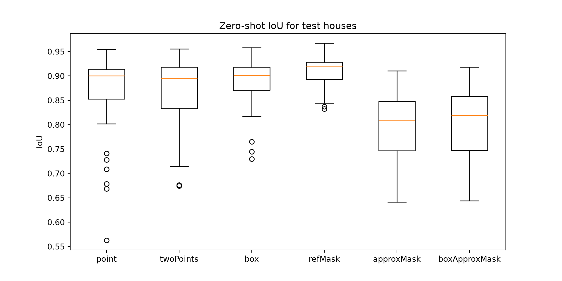
Without any training, SAM 2 produces accurate masks for most test houses using any of the prompt types. A single point and a box both produce a median IoU of approximately 0.9. A box is more consistent than a single point, which occasionally selects only part of a house or merges it with an adjacent house. Two points along the house’s axis avoid the worst single-point failures but do not improve the typical result. Providing the reference mask as a prompt produces the highest IoU but not a perfect reproduction of the reference mask, since SAM delineates the house boundaries based on the image. The approximate mask prompt substantially improves the approximate polygons, from a mean IoU of ~0.6 to ~0.8, but it is less accurate than a box. Since SAM was trained to use mask prompts in combination with its own predicted logits, binary masks are not an ideal prompt, especially ones that are larger than the feature.
Zero-shot IoU values of ~0.9 are not perfect, so it is worth examining the poorest predictions. The houses with the lowest IoU for box prompts are shown below. There are two primary sources of disagreement. First, SAM often includes the shadow along the north side of a house, which is not included in the reference polygons. Second, some of the reference polygons are offset by several pixels relative to the imagery, so even a perfect delineation of the house in the image would not perfectly match the reference polygon. The second issue is a reminder that the reference data used for assessment also contain errors, which limits the maximum IoU that can be achieved.
worst = zsDF.nsmallest(4, "box")["houseID"].tolist()
fig, axs = plt.subplots(1, 4, figsize=(20, 5))
for ax, hid in zip(axs, worst):
    img, mask, _ = chips[hid]
    showMask(ax, img, zsPreds[hid]["box"], mask, f"House {hid}, IoU: {iou(zsPreds[hid]['box'], mask):.3f}",
             box=maskToBox(mask), zoom=40)
plt.tight_layout()
plt.show()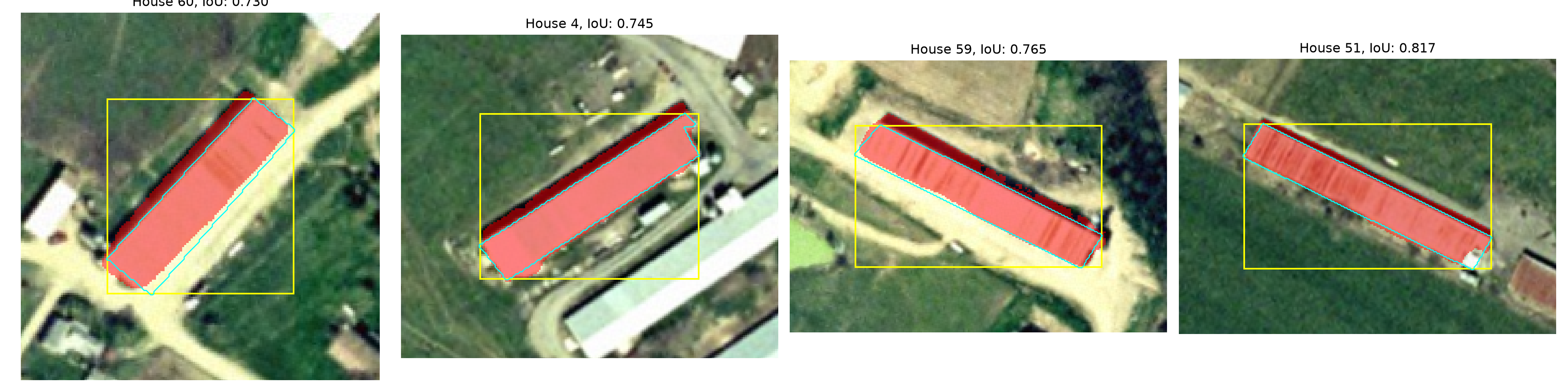
28.6 Automatic Mask Generation
The prompted workflows above require prior knowledge of where the poultry houses are. SAM can also segment an entire image without prompts. The SAM2AutomaticMaskGenerator class places a regular grid of point prompts over the image, predicts masks for every point, and filters and de-duplicates the results. Its key settings are:
-
points_per_side: the number of points along each side of the grid. More points find smaller objects but increase computation. -
pred_iou_thresh: the minimum predicted IoU for a mask to be kept. -
stability_score_thresh: the minimum stability score, which measures how much a mask changes when the threshold used to convert the predicted probabilities to a binary mask is changed. Stable masks are generally more reliable. -
min_mask_region_area: small disconnected regions and holes smaller than this area, in pixels, are removed. -
crop_n_layers: if greater than 0, the generator is also run on overlapping crops of the image, which helps with small objects in large images.
The generate() method returns a list with one dictionary per mask, containing the binary mask ("segmentation"), its area, bounding box, predicted IoU, and stability score. I create the generator using the SAM 2 model already loaded by the predictor and apply it to a 1024x1024 pixel chip centered on each test farm.
generator = SAM2AutomaticMaskGenerator(predictor.model, points_per_side=32, points_per_batch=128,
                                       pred_iou_thresh=0.8, stability_score_thresh=0.9,
                                       min_mask_region_area=100)

testFarms = [f for f in farms["farmID"] if f not in trainFarms]
farmChips, farmMasks = {}, {}
with rio.open(imgPath) as src:
    for f in testFarms:
        img, _, tr = getChip(src, farms.geometry[f], size=1024)
        with torch.inference_mode(), torch.autocast("cuda", dtype=torch.bfloat16):
            farmMasks[f] = generator.generate(img)
        farmChips[f] = (img, tr)

print(sum(len(m) for m in farmMasks.values()), farmMasks[testFarms[0]][0].keys())
1040 dict_keys(['segmentation', 'area', 'bbox', 'predicted_iou', 'point_coords', 'stability_score', 'crop_box'])28.6.1 Converting Masks to Georeferenced Polygons
To use SAM’s outputs in a GIS, the masks are converted to polygons using rasterio.features.shapes() and the chip’s transform, as we did for instance segmentation in Chapter 22 and Chapter 23. The function below converts a list of binary masks to a GeoDataFrame, storing an attribute, such as the predicted IoU, for each polygon.
def masksToGDF(masks, transform, crs, scores=None):
    rows = []
    for i, m in enumerate(masks):
        m = np.asarray(m).astype("uint8").squeeze()
        for geom, _ in features.shapes(m, mask=m == 1, transform=transform):
            rows.append({"maskID": i, "score": None if scores is None else float(scores[i]),
                         "geometry": shape(geom)})
    return gpd.GeoDataFrame(rows, geometry="geometry", crs=crs)

amgGDF = []
for f in testFarms:
    g = masksToGDF([m["segmentation"] for m in farmMasks[f]], farmChips[f][1], houses.crs,
                   scores=[m["predicted_iou"] for m in farmMasks[f]])
    g["farmID"] = f
    amgGDF.append(g)
amgGDF = gpd.GeoDataFrame(pd.concat(amgGDF, ignore_index=True), crs=houses.crs)
print(len(amgGDF))1554The automatically generated masks for one of the test farms are shown below with random colors. Automatic mask generation produces a segmentation of the image into regions, similar to the segments generated in geographic object-based image analysis (GEOBIA). The poultry houses are generally segmented well, but so are many other features, including other buildings, fields, ponds, and patches of forest. Since SAM is class-agnostic, these segments must be filtered to those that represent poultry houses.
f = houses[houses["split"] == "test"]["farmID"].value_counts().idxmax()   # test farm with most houses
img, tr = farmChips[f]
overlay = np.zeros((*img.shape[:2], 3))
rng = np.random.default_rng(1)
for m in sorted(farmMasks[f], key=lambda d: d["area"], reverse=True):
    overlay[m["segmentation"]] = rng.random(3)

fig, axs = plt.subplots(1, 2, figsize=(16, 8))
axs[0].imshow(img)
axs[1].imshow(img)
axs[1].imshow(overlay, alpha=0.5)
for ax in axs:
    ax.axis("off")
plt.tight_layout()
plt.show()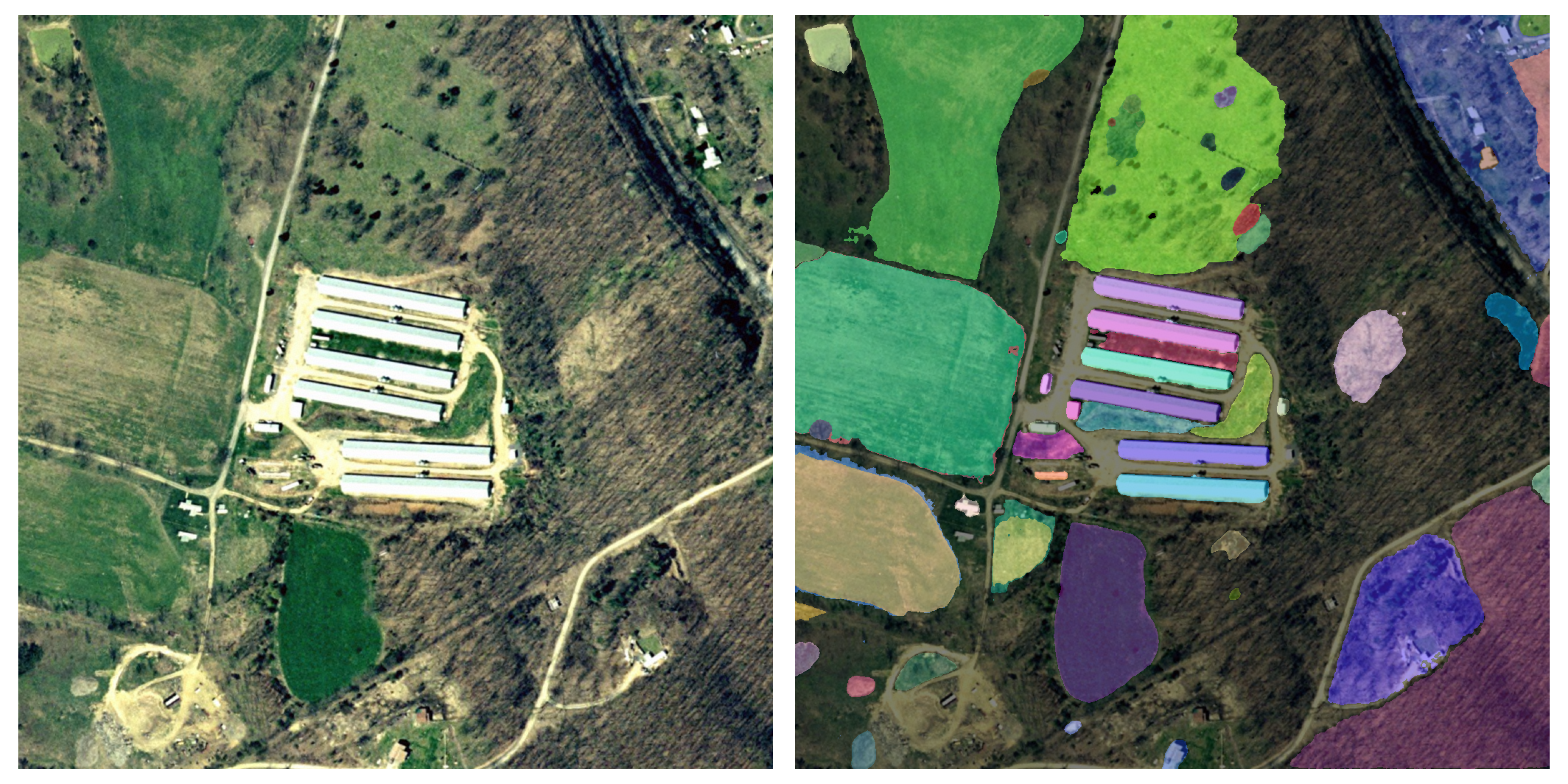
28.6.2 Filtering Segments by Shape
Poultry houses have a distinctive shape: they are long, narrow rectangles of a consistent size. So, I filter the segments using shape metrics calculated from each polygon’s minimum rotated rectangle: the length and width of the rectangle, the elongation (length divided by width), and the rectangular fit (polygon area divided by rectangle area, which is 1 for a perfect rectangle). Note that I avoid naming the columns “length” and “area” since GeoDataFrames already have length and area properties, which return the perimeter and area of each geometry, and a column with the same name could not be accessed using dot notation.
To avoid using the test data to choose the thresholds, I calculate the shape metrics for the eight training houses and set the thresholds based on their ranges with some tolerance: the area must be between half of the smallest and 1.5 times the largest training house, the length must be at least 75% of the shortest training house, the width can be at most 1.5 times the widest training house, the elongation must be at least 75% of the smallest training value, and the rectangular fit must be at least 0.8.
def shapeMetrics(gdf):
    rect = gdf.geometry.minimum_rotated_rectangle()
    sides = np.array([sorted(np.hypot(*np.diff(np.array(r.exterior.coords)[:3], axis=0).T))
                      for r in rect])
    gdf = gdf.copy()
    gdf["areaM2"] = gdf.area
    gdf["rectWidth"], gdf["rectLength"] = sides[:, 0], sides[:, 1]
    gdf["elongation"] = gdf["rectLength"] / gdf["rectWidth"]
    gdf["rectFit"] = gdf.area / rect.area
    return gdf

metricCols = ["areaM2", "rectWidth", "rectLength", "elongation", "rectFit"]
trainShape = shapeMetrics(houses[houses["split"] == "train"])
print(trainShape[metricCols].round(2))
areaM2 rectWidth rectLength elongation rectFit
5 2630.30 23.18 123.71 5.34 0.92
11 1162.33 14.07 84.10 5.98 0.98
19 2132.98 18.74 123.06 6.57 0.92
23 1417.63 16.75 95.10 5.68 0.89
33 1976.19 16.58 120.93 7.29 0.99
38 1966.70 16.45 121.63 7.39 0.98
48 1922.33 17.41 122.15 7.02 0.90
61 1969.63 18.01 121.42 6.74 0.90amgGDF = shapeMetrics(amgGDF)
isHouse = (amgGDF["areaM2"].between(trainShape["areaM2"].min() * 0.5, trainShape["areaM2"].max() * 1.5)
& (amgGDF["rectLength"] >= trainShape["rectLength"].min() * 0.75)
& (amgGDF["rectWidth"] <= trainShape["rectWidth"].max() * 1.5)
& (amgGDF["elongation"] >= trainShape["elongation"].min() * 0.75)
& (amgGDF["rectFit"] >= 0.8))
candidates = amgGDF[isHouse]
print(len(amgGDF), len(candidates))1554 44Since the farm chips can overlap, and since a grid of points can produce several similar masks for the same house, some houses are represented by more than one candidate polygon. I remove duplicates using non-maximum suppression: the candidates are sorted by their predicted IoU, and a candidate is only kept if its IoU with all previously kept candidates is below 0.5.
def polyIoU(a, b):
    return a.intersection(b).area / a.union(b).area

def polygonNMS(gdf, thresh=0.5, scoreCol="score"):
    gdf = gdf.sort_values(scoreCol, ascending=False)
    keep = []
    for i, g in gdf.geometry.items():
        if all(polyIoU(g, gdf.geometry[k]) < thresh for k in keep):
            keep.append(i)
    return gdf.loc[keep]

candidates = polygonNMS(candidates)
print(len(candidates))40I assess the results at the object level using the methods from Chapter 22. A predicted polygon is a true positive if its IoU with a reference polygon is greater than 0.5. Precision is the proportion of predicted polygons that are true positives, and recall is the proportion of reference polygons that are matched by a predicted polygon. I also calculate the mean IoU for the true positives. All reference houses on the test farms are used.
def bestIoU(geoms, refGeoms):
    out = []
    for g in geoms:
        hits = refGeoms[refGeoms.intersects(g)]
        out.append(max([polyIoU(g, r) for r in hits], default=0))
    return np.array(out)

testRef = houses[houses["split"] == "test"]
predIoU = bestIoU(candidates.geometry, testRef.geometry)
refIoU = bestIoU(testRef.geometry, candidates.geometry)
precision, recall = (predIoU > 0.5).mean(), (refIoU > 0.5).mean()
print(f"Precision: {precision:.3f}, Recall: {recall:.3f}, F1: {2 * precision * recall / (precision + recall):.3f}")
Precision: 0.975, Recall: 0.848, F1: 0.907print(f"Mean IoU of true positives: {predIoU[predIoU > 0.5].mean():.3f}")Mean IoU of true positives: 0.844fig, ax = plt.subplots(figsize=(8, 8))
img, tr = farmChips[f]
ax.imshow(img, extent=(tr.c, tr.c + img.shape[1] * tr.a, tr.f + img.shape[0] * tr.e, tr.f))
candidates[candidates["farmID"] == f].plot(ax=ax, color="red", alpha=0.4)
houses.boundary.plot(ax=ax, color="cyan", linewidth=1)
ax.set_xlim(tr.c, tr.c + img.shape[1] * tr.a)
ax.set_ylim(tr.f + img.shape[0] * tr.e, tr.f)
ax.set_axis_off()
plt.show()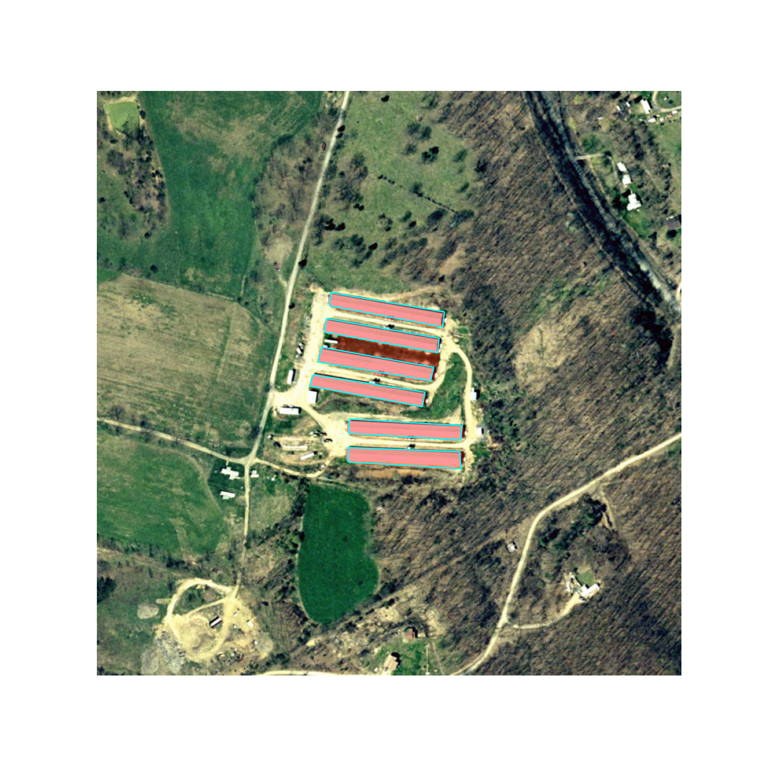
Combining zero-shot automatic mask generation with simple shape rules derived from eight example houses detects most of the test poultry houses with very few false positives. The boundaries are somewhat less accurate than when using prompts since the 1024x1024 farm chips are not upsampled. Most of the missed houses were segmented reasonably well by SAM but were removed by the shape rules because they are shorter and less elongated than any of the eight training houses. This illustrates a limitation of learning from very few examples: rules or models derived from eight houses only represent the range of houses in that small sample. Relaxing the thresholds would recover these houses at the cost of more false positives. This approach is only feasible because poultry houses have such a distinctive shape. For features that are not distinguishable by shape, the segments would need to be classified using spectral or textural characteristics, for example, using a machine learning model or a CNN, as discussed later in the chapter.
28.7 Fine-Tuning SAM 2
28.7.1 Strategy
When zero-shot performance is not adequate, SAM can be fine-tuned using labeled data. The image encoder contains most of the model’s parameters and requires substantial memory and computation to train, and with only eight training houses, there is a high risk of overfitting it. A common approach is to freeze the image encoder and fine-tune only the mask decoder, which has ~4 million parameters, using prompts derived from the labeled masks. The goal is to adjust how the decoder converts the prompts and image embeddings into masks, for example, to learn that the shadow next to a poultry house is not part of the house.
Since the image encoder is frozen, the image embeddings do not change during training. So, they can be computed once for each training chip and cached, which makes training very fast, since only the lightweight decoder is run in each iteration. A downside of caching is that augmentations that change pixel values, such as brightness or contrast adjustments, cannot be applied during training. However, I can still augment the data by caching the embeddings of flipped and rotated copies of each training chip. Using the eight combinations of 90° rotations and horizontal flips (the dihedral transformations), this produces 64 training samples from the 8 houses. Rotations are particularly appropriate for overhead imagery, in which there is no natural “up” direction, although the shadows will be on a different side of the houses in the rotated chips.
There is one detail of the SAM 2 implementation that is important here. When computing the image embedding, the forward_image() method passes the high-resolution features from the image encoder through two convolutional layers, conv_s0 and conv_s1, which are part of the mask decoder. If these layers were updated during fine-tuning, the cached features would be out of date. So, these two layers must be frozen along with the image encoder.
28.7.2 Caching the Image Embeddings
The set_image() method stores the image embedding and high-resolution features in the predictor’s _features dictionary, so I copy them from there for each transformed chip. The embedding has a shape of (256, 64, 64), and the high-resolution features have shapes of (32, 256, 256) and (64, 128, 128). I store them on the CPU as 32-bit floats, which requires approximately 1 GB of memory for the 64 samples. The masks are transformed in the same way as the chips.
def dihedral(a, k, flip):
    a = np.rot90(a, k, axes=(0, 1))
    return np.ascontiguousarray(a[:, ::-1] if flip else a)

cache = []
for hid in trainIDs:
    img, mask, _ = chips[hid]
    for k in range(4):
        for flip in (False, True):
            with torch.inference_mode(), torch.autocast("cuda", dtype=torch.bfloat16):
                predictor.set_image(dihedral(img, k, flip))
            feats = predictor._features
            cache.append({"embed": feats["image_embed"][0].float().cpu(),
                          "hr0": feats["high_res_feats"][0][0].float().cpu(),
                          "hr1": feats["high_res_feats"][1][0].float().cpu(),
                          "mask": torch.from_numpy(dihedral(mask, k, flip).astype("float32"))})
print(len(cache))
28.7.3 Dataset and Prompt Sampling
The Dataset subclass simply returns the cached features and mask for a sample. Prompts are generated randomly during training by the samplePrompts() function so that the decoder learns to respond to variable prompts as opposed to memorizing a single prompt per house. For each batch, either a box prompt or 1 to 3 random foreground points within the house are generated. Box prompts are jittered by up to 8 pixels in each direction to simulate imprecise boxes. All samples in a batch use the same prompt type and number of points so that they can be stacked into a single tensor.
SAM 2’s prompt encoder represents a box as two points with labels 2 (upper-left corner) and 3 (lower-right corner), so boxes and points can both be represented as coordinates and labels. The coordinates must be scaled from the 512x512 chip to SAM’s 1024x1024 input frame, which is handled automatically by the predict() method but must be done manually here.
class CachedFeatures(Dataset):
    def __init__(self, cache):
        self.cache = cache

    def __len__(self):
        return len(self.cache)

    def __getitem__(self, idx):
        d = self.cache[idx]
        return d["embed"], d["hr0"], d["hr1"], d["mask"]

def samplePrompts(masks, mode, nPts=1, jitter=8):
    # masks: (B, H, W); returns coordinates (B, N, 2) in SAM's 1024x1024 frame and labels (B, N)
    B, H, W = masks.shape
    coords, labels = [], []
    for b in range(B):
        rows, cols = torch.where(masks[b] > 0)
        if mode == "box":
            j = torch.randint(-jitter, jitter + 1, (4,), device=masks.device)
            c = torch.stack([torch.stack([cols.min() + j[0], rows.min() + j[1]]),
                             torch.stack([cols.max() + j[2], rows.max() + j[3]])]).float()
            l = torch.tensor([2, 3], device=masks.device)
        else:
            idx = torch.randint(0, len(rows), (nPts,), device=masks.device)
            c = torch.stack([cols[idx], rows[idx]], dim=1).float()
            l = torch.ones(nPts, dtype=torch.long, device=masks.device)
        coords.append(c.clamp(0, W - 1) * (1024 / W))
        labels.append(l)
    return torch.stack(coords), torch.stack(labels).int()
28.7.4 LightningModule
The LightningModule receives the SAM 2 model and keeps references to its prompt encoder and mask decoder. The prompt encoder and the decoder’s conv_s0 and conv_s1 layers are frozen, and only the remaining decoder parameters are passed to the optimizer. The forward() method mirrors the steps in the predictor’s internal _predict() method: the prompts are embedded, and the decoder combines the prompt embeddings, the image embedding, and the high-resolution features to predict a 256x256 mask of logits and a predicted IoU score. Since one prompt is provided per image, repeat_image=False. Note that Lightning does not change whether modules are in training or evaluation mode, and the predictor’s SAM 2 model is in evaluation mode, which Lightning reports in its model summary. SAM 2’s decoder does not use dropout or batch normalization, so this only affects one behavior: in evaluation mode, when a single point is provided and a single mask is requested, the decoder selects the most stable of its candidate masks. Keeping the decoder in evaluation mode means it is trained the same way it is used by the predictor.
The loss is the sum of three components. The predicted logits are upsampled to 512x512 and compared to the reference mask using binary cross entropy and Dice loss (Chapter 4), which is the combination used to train SAM. SAM also predicts the IoU of each mask, which is used to rank candidate masks, so the mean squared error between the predicted IoU and the actual IoU of the predicted mask is also included, as in the original SAM training. I use a small learning rate, since the goal is to adjust, not replace, the pre-trained decoder.
class SAMDecoderTuner(L.LightningModule):
    def __init__(self, sam, lr=5e-5):
        super().__init__()
        self.promptEncoder = sam.sam_prompt_encoder
        self.decoder = sam.sam_mask_decoder
        self.lr = lr
        frozen = (list(self.promptEncoder.parameters()) + list(self.decoder.conv_s0.parameters())
                  + list(self.decoder.conv_s1.parameters()))
        for p in frozen:
            p.requires_grad = False

    def forward(self, embed, highRes, coords, labels):
        sparse, dense = self.promptEncoder(points=(coords, labels), boxes=None, masks=None)
        lowRes, iouPred, _, _ = self.decoder(image_embeddings=embed,
                                             image_pe=self.promptEncoder.get_dense_pe(),
                                             sparse_prompt_embeddings=sparse,
                                             dense_prompt_embeddings=dense,
                                             multimask_output=False, repeat_image=False,
                                             high_res_features=highRes)
        return lowRes, iouPred

    def training_step(self, batch, batch_idx):
        embed, hr0, hr1, mask = batch
        mode = "box" if torch.rand(1) < 0.5 else "point"
        coords, labels = samplePrompts(mask, mode, nPts=int(torch.randint(1, 4, (1,))))
        lowRes, iouPred = self(embed, [hr0, hr1], coords, labels)
        logits = F.interpolate(lowRes, size=mask.shape[-2:], mode="bilinear", align_corners=False)[:, 0]

        prob = torch.sigmoid(logits)
        bce = F.binary_cross_entropy_with_logits(logits, mask)
        inter = (prob * mask).sum((1, 2))
        dice = 1 - (2 * inter + 1) / (prob.sum((1, 2)) + mask.sum((1, 2)) + 1)

        pred = (logits > 0).float()
        trueIoU = (pred * mask).sum((1, 2)) / ((pred + mask).clamp(max=1).sum((1, 2)) + 1e-6)
        iouLoss = F.mse_loss(iouPred[:, 0].float(), trueIoU)

        loss = bce + dice.mean() + iouLoss
        self.log_dict({"train_loss": loss, "train_iou": trueIoU.mean()}, on_step=False, on_epoch=True)
        return loss

    def configure_optimizers(self):
        params = [p for p in self.decoder.parameters() if p.requires_grad]
        return torch.optim.AdamW(params, lr=self.lr, weight_decay=1e-4)
28.7.5 Training
I train for 40 epochs with a batch size of 8 using bfloat16 mixed precision. With 64 cached samples, each epoch consists of 8 iterations. There are too few labeled houses to hold some out for validation, so the number of epochs and the learning rate are fixed in advance, and the model is assessed using the test houses after training. At the end of fit(), Lightning moves the LightningModule to the CPU. Since the prompt encoder and mask decoder are shared with the predictor’s SAM 2 model, they are also moved, while the image encoder remains on the GPU. So, I move the entire SAM 2 model back to the GPU after training. Finally, I save the state dictionary of the fine-tuned mask decoder, which is much smaller than the entire model.
L.seed_everything(42)
trainDL = DataLoader(CachedFeatures(cache), batch_size=8, shuffle=True)
tuner = SAMDecoderTuner(predictor.model, lr=5e-5)

trainer = L.Trainer(max_epochs=40, accelerator="gpu", devices=1, precision="bf16-mixed",
                    logger=CSVLogger("data/output/", name="samPoultry"),
                    enable_checkpointing=False)
trainer.fit(tuner, train_dataloaders=trainDL)

predictor.model.to(device).eval()
torch.save(predictor.model.sam_mask_decoder.state_dict(),
           "data/output/samPoultryDecoder.pt")
Caching the embeddings took less than a minute, and training took about 30 seconds on my machine with a single GPU. If you do not want to or cannot train the model, the fine-tuned decoder parameters and training log have been provided with the text. The training loss and the IoU of the predicted training masks are plotted below. The training IoU increases from ~0.90 to ~0.95.
resultsDF = pd.read_csv("data/models/samPoultryLogs.csv")

fig, axs = plt.subplots(1, 2, figsize=(12, 4))
resultsDF.plot(x="epoch", y="train_loss", ax=axs[0], legend=False, title="Training loss")
resultsDF.plot(x="epoch", y="train_iou", ax=axs[1], legend=False, title="Training IoU")
plt.show()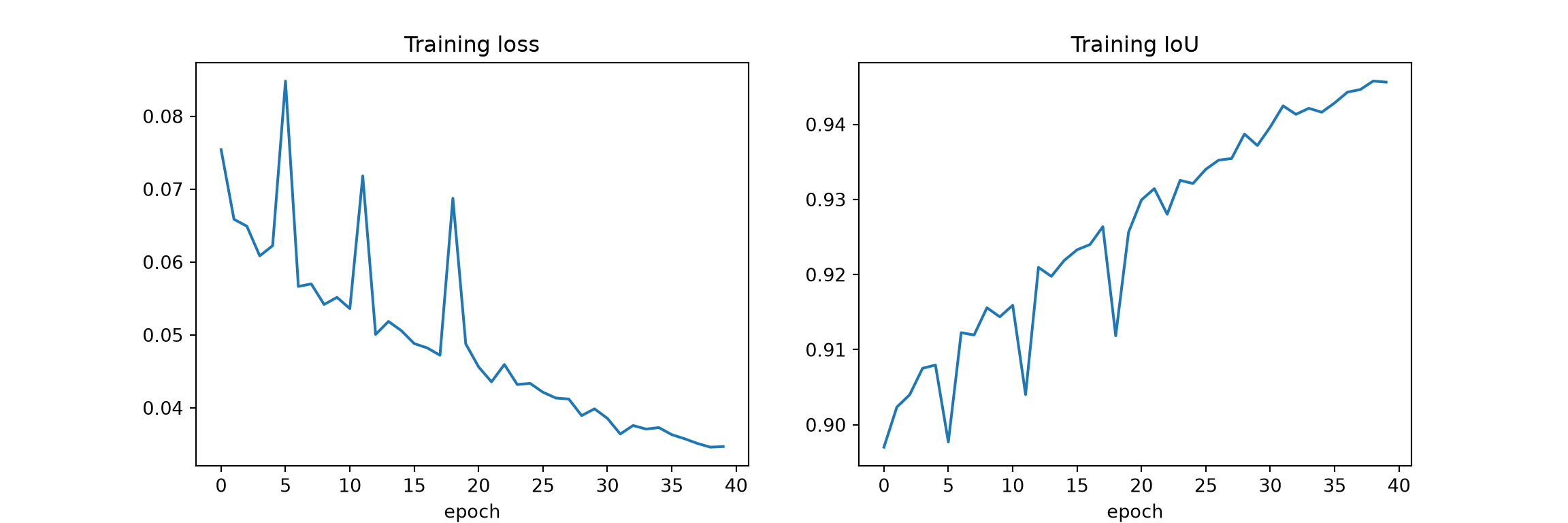
28.7.6 Assessing the Fine-Tuned Model
To use the fine-tuned model, I load the saved parameters into the predictor’s mask decoder. Since only the decoder changed, the predictor can be used exactly as before. I then apply the point, two-point, and box prompts to the test houses, which were not used for fine-tuning. The mask prompts are not included, since mask prompts were not used during fine-tuning.
predictor.model.sam_mask_decoder.load_state_dict(
    torch.load("data/models/samPoultryDecoder.pt", map_location=device))
predictor.model.eval()

ftTypes = ["point", "twoPoints", "box"]
ftDF, ftPreds = assessPrompts(predictor, testIDs, ftTypes)

compareDF = pd.DataFrame({"zeroShotMean": zsDF[ftTypes].mean(), "fineTunedMean": ftDF[ftTypes].mean(),
                          "zeroShotMin": zsDF[ftTypes].min(), "fineTunedMin": ftDF[ftTypes].min()})
compareDF.round(3)
zeroShotMean fineTunedMean zeroShotMin fineTunedMin
point 0.868 0.872 0.563 0.553
twoPoints 0.871 0.877 0.675 0.655
box 0.887 0.893 0.730 0.802fig, axs = plt.subplots(1, 3, figsize=(15, 5))
for ax, p in zip(axs, ftTypes):
ax.scatter(zsDF[p], ftDF[p])
ax.plot([0.5, 1], [0.5, 1], color="gray", linestyle="--")
ax.set_xlabel("Zero-shot IoU")
ax.set_ylabel("Fine-tuned IoU")
ax.set_title(p)
plt.tight_layout()
plt.show()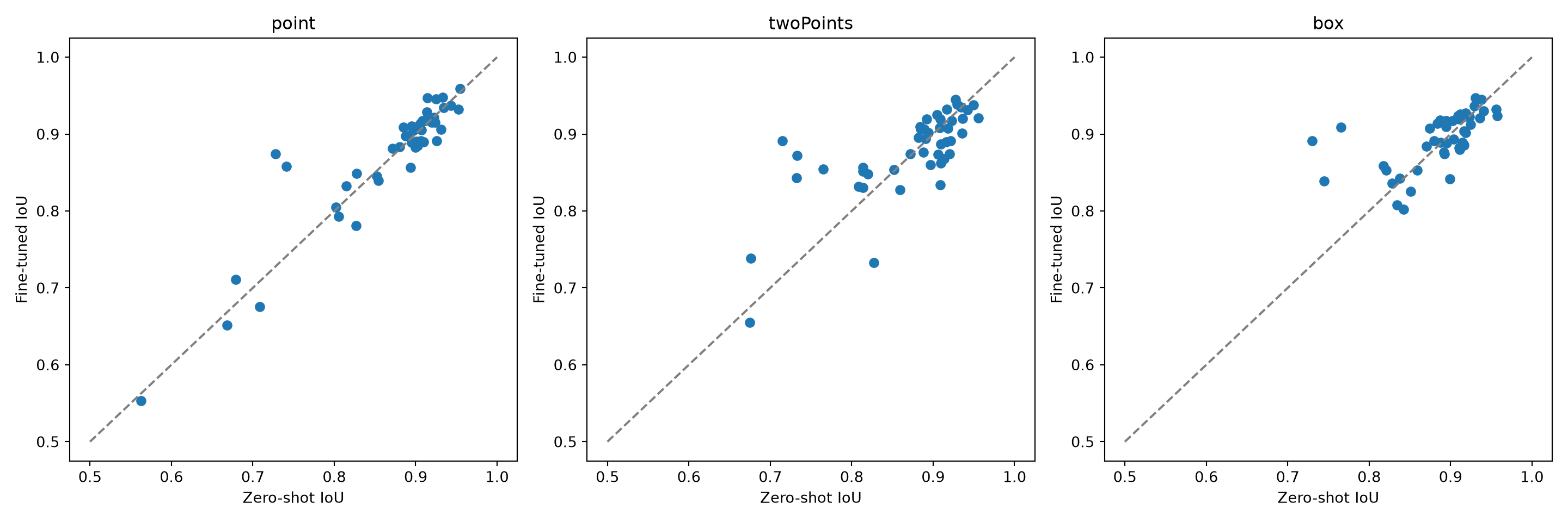
Each point in the plots above is a test house, and points above the dashed line were improved by fine-tuning. Fine-tuning with eight houses produces only a small increase in the mean IoU, since the zero-shot model already performed well for most houses and the remaining disagreement is partially due to errors in the reference polygons. For box prompts, about as many houses were slightly degraded as were improved. However, fine-tuning reduced the largest errors, so the minimum IoU and the variability between houses decreased. The improved houses include several where the zero-shot model included the shadow, as shown below for the houses with the lowest zero-shot IoU for box prompts. With so few training samples, the results of fine-tuning will also vary depending on which houses are selected and the random prompts generated during training.
fig, axs = plt.subplots(2, 4, figsize=(20, 10))
for j, hid in enumerate(worst):
    img, mask, _ = chips[hid]
    showMask(axs[0, j], img, zsPreds[hid]["box"], mask, f"House {hid} zero-shot, IoU: {zsDF.set_index('houseID').loc[hid, 'box']:.3f}",
             zoom=40)
    showMask(axs[1, j], img, ftPreds[hid]["box"], mask, f"House {hid} fine-tuned, IoU: {ftDF.set_index('houseID').loc[hid, 'box']:.3f}",
             zoom=40)
plt.tight_layout()
plt.show()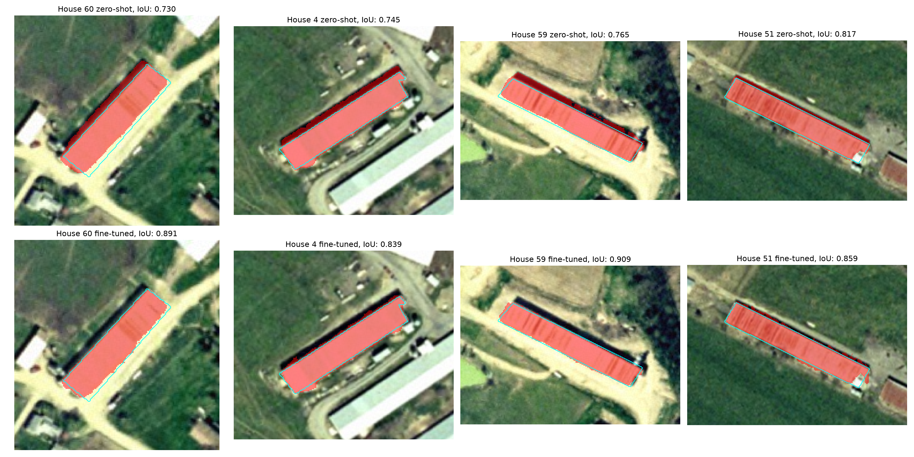
28.7.7 Mapping the Test Houses
Finally, I convert the fine-tuned box predictions for the test houses to georeferenced polygons and save them to a GeoPackage. Since a mask may be converted to several polygons, for example, when a narrow part of the mask is only connected diagonally, I dissolve the polygons for each house into a single multipart feature. I then compare the predicted polygons to the reference polygons using IoU and area. The area of each house might be used, for example, to estimate the number of birds and amount of litter produced at each farm.
predGDF = []
for hid in testIDs:
    g = masksToGDF([ftPreds[hid]["box"]], chips[hid][2], houses.crs)
    g = g.dissolve().drop(columns=["maskID", "score"])
    g["houseID"] = hid
    predGDF.append(g)
predGDF = gpd.GeoDataFrame(pd.concat(predGDF, ignore_index=True), crs=houses.crs)

refGeoms = houses.set_index("houseID").geometry
predGDF["iou"] = [polyIoU(g, refGeoms[h]) for g, h in zip(predGDF.geometry, predGDF["houseID"])]
predGDF["predArea"] = predGDF.area
predGDF["refArea"] = [refGeoms[h].area for h in predGDF["houseID"]]
predGDF.to_file("data/output/poultryHousesSAM.gpkg")

print(predGDF[["iou", "predArea", "refArea"]].describe().round(2))
iou predArea refArea
count 46.00 46.00 46.00
mean 0.89 1747.85 1690.82
std 0.04 490.06 508.29
min 0.80 489.04 427.27
25% 0.88 1447.16 1383.37
50% 0.90 1906.56 1833.34
75% 0.92 2060.60 1997.66
max 0.94 2624.33 2937.10print(np.corrcoef(predGDF["predArea"], predGDF["refArea"])[0, 1])0.9615174691166253fig, ax = plt.subplots(figsize=(8, 8))
img, tr = farmChips[f]
ax.imshow(img, extent=(tr.c, tr.c + img.shape[1] * tr.a, tr.f + img.shape[0] * tr.e, tr.f))
predGDF.plot(ax=ax, color="red", alpha=0.4)
houses.boundary.plot(ax=ax, color="cyan", linewidth=1)
ax.set_xlim(tr.c, tr.c + img.shape[1] * tr.a)
ax.set_ylim(tr.f + img.shape[0] * tr.e, tr.f)
ax.set_axis_off()
plt.show()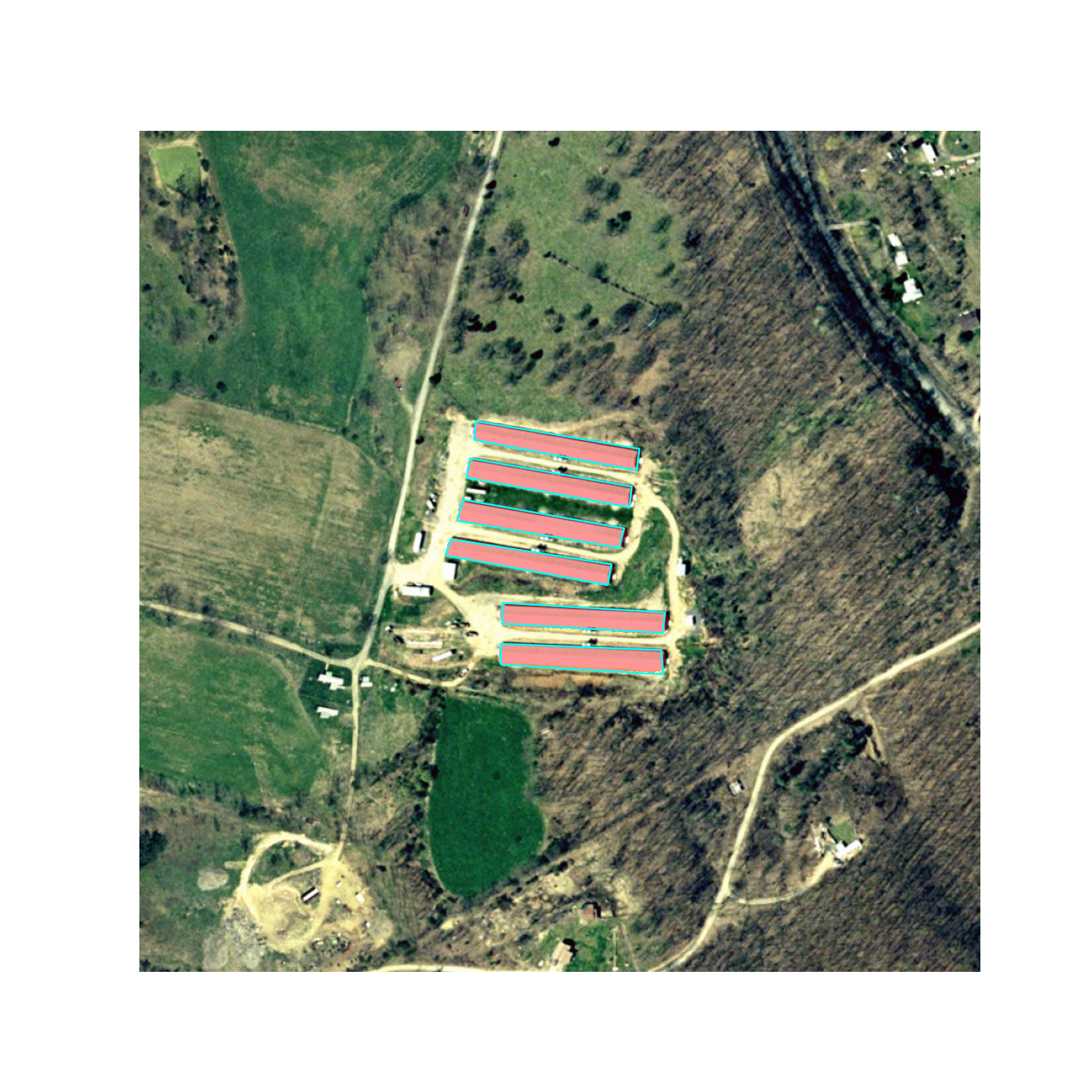
28.8 Processing Large Images
In this chapter, I extracted chips around known houses and farms. To map an entire image, the image must be processed as tiles. SAM 2 resizes each input image to 1024x1024 pixels internally, so providing a much larger image would reduce its effective spatial resolution and cause small features to be missed. As with the instance segmentation models in Chapter 23, objects that cross tile boundaries may be split or detected in multiple overlapping tiles, so tiles are generally overlapped and the resulting polygons are merged or deduplicated, for example, using the polygonNMS() function defined above. The code below loops over overlapping tiles, applies automatic mask generation, and combines the polygons from each tile. For imagery that is not already 8-bit RGB, each tile would also need to be converted. If a percentile stretch is used for this conversion, it should be calculated for the entire image and applied to each tile, since calculating it separately for each tile can cause differences in appearance between tiles.
def samTiles(path, generator, tile=1024, overlap=256):
    gdfs = []
    with rio.open(path) as src:
        H, W, crs = src.height, src.width, src.crs
        step = tile - overlap
        for r in range(0, max(H - overlap, 1), step):
            for c in range(0, max(W - overlap, 1), step):
                win = Window(c, r, min(tile, W - c), min(tile, H - r))
                img = np.transpose(src.read([1, 2, 3], window=win), (1, 2, 0))
                with torch.inference_mode(), torch.autocast("cuda", dtype=torch.bfloat16):
                    ms = generator.generate(img)
                if ms:
                    gdfs.append(masksToGDF([m["segmentation"] for m in ms], src.window_transform(win),
                                           crs, scores=[m["predicted_iou"] for m in ms]))
    return gpd.GeoDataFrame(pd.concat(gdfs, ignore_index=True), crs=crs) if gdfs else None

allSegments = samTiles(imgPath, generator)
houseCandidates = polygonNMS(shapeMetrics(allSegments)[...])   # apply the shape filter
The full SAMB image used here is 19,244 x 24,146 pixels, which corresponds to about 800 tiles of 1024x1024 pixels with 256 pixels of overlap. At roughly 4 seconds per tile on my machine, this would take nearly an hour. When features are sparse, it is more efficient to first identify the tiles likely to contain features of interest, for example, using a CNN scene classifier, and only apply SAM to those tiles.
28.9 Combining SAM with Trained Models
Since SAM is class-agnostic, it is most useful for geospatial mapping when combined with information about which features are of interest. In this chapter, we used prompts derived from existing data and shape rules applied to automatically generated segments. Other strategies include:
- Prompts from a detection model: the bounding boxes predicted by an object detection model, such as the box branch of Mask R-CNN (Chapter 23), are used as box prompts, and SAM refines the masks. This combines the detector’s knowledge of what to detect with SAM’s ability to delineate boundaries.
- Prompts from a semantic segmentation model: points are sampled from the regions predicted to be a class of interest by a semantic segmentation model, such as those trained in Chapter 16 and Chapter 21, and SAM separates them into individual objects. This would be useful for separating adjacent poultry houses that a semantic segmentation model predicts as a single region.
- Classifying SAM segments: segments from automatic mask generation are classified using another model, for example, a CNN scene classifier (Chapter 11) applied to each segment’s bounding box or a machine learning model applied to summary statistics calculated within each segment, similar to GEOBIA.
# Example: refine boxes predicted by a trained Mask R-CNN model using SAM 2
maskrcnn.eval()
imgTensor = torch.from_numpy(img).permute(2, 0, 1).float().div(255).to(device)
with torch.no_grad():
    det = maskrcnn([imgTensor])[0]
keep = det["scores"] > 0.5
boxes = det["boxes"][keep].cpu().numpy()

with torch.inference_mode(), torch.autocast("cuda", dtype=torch.bfloat16):
    predictor.set_image(img)
    refined, scores, _ = predictor.predict(box=boxes, multimask_output=False)
28.10 Limitations
SAM performed well for poultry houses, which have clear boundaries and strong contrast with their surroundings. It generally performs well for other features with these characteristics, such as other buildings, agricultural fields, and water bodies, and less well for features with gradual or ambiguous boundaries, such as vegetation communities, soils, or geomorphic features in terrain data. Some important limitations are:
- Three-band, 8-bit input: multispectral, hyperspectral, SAR, and terrain data must be reduced to three bands and 8-bit values, which discards information.
- Domain shift: SAM was trained primarily on natural photographs taken from the ground. The overhead perspective, spatial resolution, and appearance of remotely sensed imagery differ from these photographs. Features such as shadows, which are common in aerial imagery, may be included in or excluded from masks inconsistently.
- No classes: SAM must be combined with prompts, rules, or other models to produce thematic maps.
- Scale: small features, such as individual trees in moderate-resolution imagery, may be missed, while large features may be split.
- Computation: the large image encoders require a GPU and significant memory, which can make processing large areas slow.
Beyond fine-tuning the mask decoder, as demonstrated above, parameter-efficient methods, such as adapters or low-rank adaptation (LoRA), which train a small number of added parameters within the image encoder, can adapt SAM’s image features to a new domain. These approaches require more labeled data and computation than decoder fine-tuning, and the image embeddings cannot be cached since they change during training.
Regardless of how SAM is used, its outputs should be assessed using withheld reference data, just like any other model. Zero-shot does not mean error-free, and the quality of SAM’s outputs can vary substantially between images and features. As we saw with the poultry houses, the reference data should also be scrutinized, since errors in the reference data limit the accuracy that can be measured.
28.11 Other Geospatial Foundation Models
SAM is a segmentation model, but other foundation models are designed to be fine-tuned for classification, semantic segmentation, regression, and change detection. Geospatial foundation models, such as Prithvi, accept multispectral and multitemporal inputs, which addresses some of the limitations of SAM. These models are generally fine-tuned by attaching a task-specific head or decoder to the pre-trained encoder and training with labeled data, which is the same process we used to fine-tune the FCMAE encoder in Chapter 27. Libraries such as TerraTorch provide tools for fine-tuning geospatial foundation models, and TorchGeo provides pre-trained weights for many remote sensing datasets. For applying SAM and other foundation models to geospatial data with high-level tools, see the GeoAI with Python text and the geoai and segment-geospatial packages by Qiusheng Wu.
28.12 Concluding Remarks
In this chapter, we explored foundation models and applied SAM 2 to the problem of mapping poultry houses from leaf-off aerial imagery. Without any training, SAM 2 delineated most poultry houses accurately using point, box, and mask prompts, and automatic mask generation combined with shape rules derived from eight example houses detected most of the houses without prompts. Fine-tuning the mask decoder using eight labeled houses, with the image encoder frozen and the image embeddings cached, was fast and reduced the largest errors for houses not used in training, although the gain in mean IoU was small since zero-shot performance was already high. We also converted SAM’s outputs to georeferenced polygons, discussed processing large images as tiles and combining SAM with trained models, and considered SAM’s limitations. Foundation models are developing rapidly, and new models and versions are released frequently. However, the skills developed throughout this text, including preparing geospatial data, understanding model architectures, fine-tuning models, and rigorously assessing their outputs, will remain essential for using them effectively.
28.13 Questions
- What is a foundation model? Describe three characteristics that distinguish foundation models from the models trained earlier in this text.
- Describe the three components of the Segment Anything Model. Why can many prompts be applied to the same image efficiently?
- Why does SAM return multiple candidate masks for a single point prompt? Using the poultry house example, explain why the mask with the highest predicted IoU score is not always the best match to the feature of interest.
- Why might an axis-aligned bounding box be a poor prompt for a long, narrow feature that is oriented diagonally? How could this problem be reduced?
- What does it mean that SAM is class-agnostic? Explain how shape rules were used to identify poultry houses among the outputs of automatic mask generation and why the thresholds were derived from the training houses as opposed to the test houses.
- Why were the houses grouped into farms before the training and test houses were selected?
- Explain why the image embeddings could be cached when fine-tuning SAM 2’s mask decoder. What are the advantages and limitations of caching, and why must the decoder’s
conv_s0andconv_s1layers be frozen? - Fine-tuning with eight houses only slightly increased the mean IoU for the test houses. Discuss two reasons for this result and how you would determine whether fine-tuning is worthwhile for a new mapping problem.