import numpy as np
import pandas as pd
import matplotlib.pyplot as plt
import rasterio as rio
from rasterio import features
from rasterio.windows import from_bounds
import geopandas as gpd
from shapely.geometry import shape, box
from scipy import ndimage as ndi
from skimage.segmentation import watershed

import torch
import torch.nn as nn
import torch.nn.functional as F
from torch.utils.data import Dataset, DataLoader
import torchmetrics as tm
import albumentations as A
import lightning as L
from lightning.pytorch.callbacks import ModelCheckpoint
from lightning.pytorch.loggers import CSVLogger
from torchinfo import summary
from terrainseg import lspModule

device = torch.device("cuda:0" if torch.cuda.is_available() else "cpu")22 Instance Segmentation with UNet-ID
22.1 Introduction
So far, we have performed semantic segmentation, in which each pixel is assigned to a class. Semantic segmentation tells us where features are, but not how many there are or which pixels belong to which feature. If two features touch or are separated by only a pixel or two, a semantic segmentation will often merge them into a single region. Instance segmentation goes a step further: each pixel is assigned to a class and to an individual object, or instance. For many geospatial applications, such as counting buildings, estimating building sizes, inventorying trees, or mapping individual landslides or ponds, the instances are what matter.
There are two general approaches to instance segmentation. Detection-based methods, such as Mask R-CNN, which we explore in Chapter 23, first detect objects using bounding boxes and then predict a mask within each box. Segmentation-based methods start from a semantic segmentation architecture and modify the labels and outputs so that individual objects can be separated in a post-processing step. In this chapter, we build a segmentation-based method from scratch: UNet-ID, which was proposed by Wagner et al. (2020) for extracting individual buildings from very high spatial resolution satellite imagery.
Wagner, F.H., Dalagnol, R., Tarabalka, Y., Segantine, T.Y., Thomé, R. and Hirye, M.C., 2020. “U-Net-Id, an instance segmentation model for building extraction from satellite images—Case study in the Joanópolis City, Brazil.” Remote Sensing, 12(10), p.1544. https://doi.org/10.3390/rs12101544
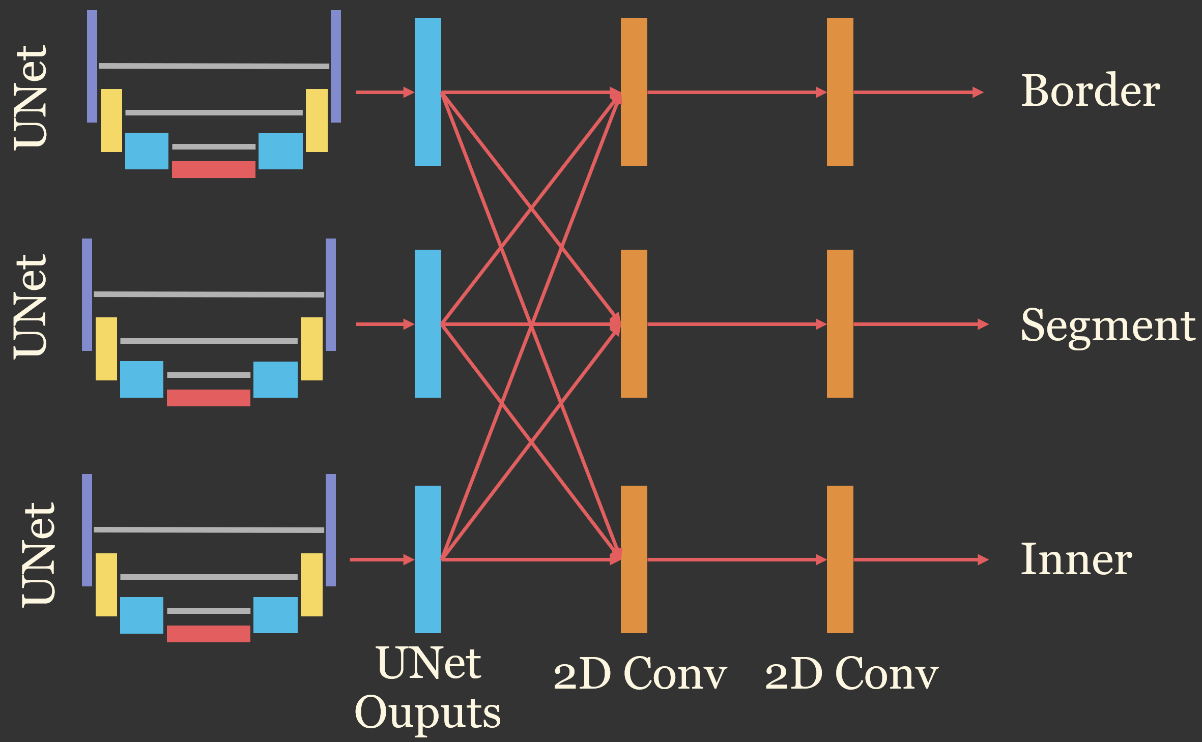
The key idea of UNet-ID is that touching objects can be separated if the model also learns to predict the border of each object and a shrunken inner segment of each object. The inner segments of neighboring objects do not touch, so each inner segment can be labeled as a separate object and then grown back to the full object extent. UNet-ID predicts three masks:
- The full object segment.
- The object border, which is a band of pixels along the edge of each object.
- The inner object segment, which is each object shrunk inward from its edges.
In the original paper, the model was trained using WorldView-3 RGB imagery with a spatial resolution of 0.3 m. Image tiles of 256x256 pixels were used. The inner segment was generated by shrinking each building by 2 pixels, and the border was defined as a band extending 4 pixels outside and 3 pixels inside each building’s outline. So, the three masks overlap. The architecture consists of three separate UNets, one for each mask. The outputs of the three UNets are concatenated, and each output path then applies two convolutional layers, with 64 and 32 filters, before making its final prediction. This allows each prediction to use the information from all three UNets. In this chapter, I implement this design using the UNet built in Chapter 15 as the basis for each of the three branches. To keep the implementation simple, the outputs have the same size as the input chips. The original implementation cropped the 256x256 input tiles to 160x160 outputs to avoid edge effects, which is similar to the cropping used for spatial predictions in Chapter 19. You should consult the paper and the authors’ code, which is available at https://doi.org/10.5281/zenodo.3716070, for the exact implementation details.
The UNet-ID architecture is conceptualized in Figure 22.1. Three UNet branches are applied to the input image. The outputs of all three branches are passed to each of three output paths, so each mask is predicted using the information learned by all of the branches. Each path then applies two 2D convolutional layers to predict the border, full segment, or inner segment mask.
The general workflow is:
- Rasterize object polygons to an instance raster, in which each object has a unique integer ID.
- Derive the full, border, and inner masks from the instance raster.
- Train UNet-ID to predict the three masks.
- Separate the predicted objects into instances in a post-processing step.
- Assess the results at the pixel-level and the object-level.
The example in this chapter maps individual valley fill faces, the engineered slopes created when mining spoil is placed in valleys adjacent to mountaintop removal coal mines, using data derived from the vfillDL dataset introduced in Chapter 20. The same data are used for Mask R-CNN in Chapter 23, so the results of the two approaches can be compared.
22.2 The Valley Fill Instance Dataset
The vfillDL dataset provides lidar-derived digital terrain models (DTMs) with a 2 m cell size and polygons of the valley fill faces for several study areas in West Virginia, Kentucky, and Virginia. To keep the example manageable, I only use three of the study areas: KY1 for training, KY2 for validation, and VA1 for testing. Since the three areas are geographically separated, the validation and test data provide an assessment of how well the model generalizes to new areas. This is a fairly small training set: KY1 contains 553 valley fill faces. Adding the larger West Virginia training area would likely improve the results, so the model trained here should not be considered optimal.
I created the image chips and instance chips ahead of time; the resulting dataset, vfillInst, is provided as a separate download (see Table 2). The DTM and polygons for VA1, which are used to map a larger area at the end of the chapter, are part of the vfillDL dataset. Each chip is 512x512 cells and contains three land surface parameters (LSPs) calculated from the DTM using the lspModule class from the terrainseg package: a hillslope-scale topographic position index (TPI), the square root of slope, and a multidirectional hillshade. All three are already scaled from 0 to 1. The LSPs were calculated for 640x640 cell windows, and 64 cells were trimmed from each side, since the convolutions used to calculate the LSPs pad the edges of the input with zeros and produce incorrect values near the edges. The radii that define the moving windows used by lspModule are specified as numbers of cells, as opposed to map units. The default radii were designed for data with a 1 m cell size, so I halved them for these 2 m data; otherwise, the windows would cover twice the intended distance, and roughly 20% of the TPI values would be clipped at the ±10 m limits used to rescale the TPI. I use the same settings when predicting to new areas below.
The chips were generated as follows:
- Training: one chip centered on each valley fill face in KY1. All valley fill faces that fall within a chip are included in its instance chip, so a face can occur in several overlapping chips. Centering the chips on the objects guarantees that every valley fill face is fully contained in at least one chip.
- Validation and testing: a grid of non-overlapping chips covering KY2 and VA1. Chips centered on the objects would make the assessment overly optimistic, since in practice the model must be applied to the entire landscape.
- Background: chips that contain no valley fill faces were sampled from the grid in each area, with one background chip for every two chips containing valley fill faces. These help the model learn to avoid false positives on the mine benches, roads, and other features that resemble valley fill faces.
Each partition is described by a CSV file that lists the chip names, whether the chip contains valley fill faces (“Positive”) or not (“Background”), and the number of instances.
ImportantData Location
This chapter uses the vfillInst dataset, which is provided as a separate download (vfillInst.zip) in the download menu in the sidebar, and the VA1 DTM and polygons from the vfillDL dataset, which is too large to include in the book download and must be downloaded from the source listed in Table 2. By default, the code expects the uncompressed vfillInst and vfillDL folders to be saved in the data/files folder (data/files/vfillInst and data/files/vfillDL). If you saved the data elsewhere, set folder below and dtmPath and the reference polygon path in the section on predicting to geospatial data to the correct locations on your machine.
# Set this to the location of the uncompressed vfillInst folder on your machine.
folder = "data/files/vfillInst/"
trainDF = pd.read_csv(folder + "trainDF.csv")
valDF = pd.read_csv(folder + "valDF.csv")
testDF = pd.read_csv(folder + "testDF.csv")

pd.DataFrame({split: [len(df), (df["division"] == "Positive").sum(), df["nInst"].sum()]
              for split, df in zip(["train", "val", "test"], [trainDF, valDF, testDF])},
             index=["Chips", "Positive chips", "Instances"])
train val test
Chips 795 180 193
Positive chips 533 119 127
Instances 1574 214 19122.3 Preparing the Labels
22.3.1 Instance Rasters
Object outlines are commonly available as vector polygons. To generate instance labels, each polygon is burned into a raster aligned with the image using a unique integer value. The function below assigns a sequential ID to each polygon and uses rasterio.features.rasterize() to burn the IDs into a grid with the same transform and dimensions as an image. Background cells are coded to 0. The instance chips in the vfillInst dataset were created in this way, so I do not need to run this function here; it is used below to create a reference instance raster for a larger area.
def makeInstanceRaster(polys, outShape, transform):
    shapes = ((geom, i + 1) for i, geom in enumerate(polys.geometry))
    return features.rasterize(shapes, out_shape=outShape, transform=transform,
                              fill=0, dtype="int32")
22.3.2 Deriving the Three Masks
From the instance raster, the three masks are derived using morphological operations, which are applied separately to each object so that the masks of neighboring objects are calculated independently. Erosion shrinks a binary region by removing pixels along its edges, and dilation grows it by adding pixels. For each object:
- The full segment is the object’s pixels.
- The inner segment is the object eroded by
innerErodepixels. - The border is the object dilated by
borderOutpixels minus the object eroded byborderInpixels, which yields a band extendingborderOutpixels outside andborderInpixels inside the outline.
The results for all objects are combined into three binary masks. Note that the border of one object can extend over a neighboring object. This is intended: the border marks the boundaries between objects, which is what allows touching objects to be separated. Small objects may disappear entirely when eroded, so their inner segments will be empty; I keep at least the object’s center pixel in such cases.
The number of pixels used for each operation should be adjusted based on the spatial resolution of the data and the typical size of and spacing between objects. The values used in the original paper (2, 4, and 3 pixels) correspond to distances of less than 1.5 m at 0.3 m resolution, which suits buildings that are often only a few meters apart. The valley fill faces are much larger, with a median area of roughly 4,600 cells, or 1.8 ha, and they do not touch each other. I use 3 pixels for all three settings, which corresponds to 6 m at 2 m resolution. This produces inner segments that are well separated from the outlines and borders that are wide enough to be learned reliably.
def makeUNetIDMasks(inst, innerErode=3, borderOut=3, borderIn=3):
    full = inst > 0
    inner = np.zeros_like(full)
    border = np.zeros_like(full)
    for objID, sl in enumerate(ndi.find_objects(inst), start=1):
        if sl is None:
            continue
        # Expand the bounding slice so dilation is not clipped
        sl = tuple(slice(max(s.start - borderOut - 1, 0), s.stop + borderOut + 1) for s in sl)
        obj = inst[sl] == objID
        objInner = ndi.binary_erosion(obj, iterations=innerErode)
        if not objInner.any():                      # keep small objects represented
            cy, cx = [int(round(c)) for c in ndi.center_of_mass(obj)]
            objInner[cy, cx] = True
        objBorder = ndi.binary_dilation(obj, iterations=borderOut) & \
                    ~ndi.binary_erosion(obj, iterations=borderIn)
        inner[sl] |= objInner
        border[sl] |= objBorder
    return np.stack([full, border, inner]).astype("uint8")   # (3, H, W)
To visualize the masks for a chip, I plot the hillshade band, the instance chip, and the three derived masks side by side.
chpN = trainDF.loc[trainDF["nInst"] >= 3, "chpN"].iloc[0]
with rio.open(f"{folder}train/images/{chpN}") as src:
    hs = src.read(3)
with rio.open(f"{folder}train/masks/{chpN}") as src:
    inst = src.read(1).astype("int32")
masks = makeUNetIDMasks(inst)

fig, axs = plt.subplots(1, 5, figsize=(18, 4))
axs[0].imshow(hs, cmap="gray", vmin=np.quantile(hs, 0.01), vmax=np.quantile(hs, 0.99))
axs[0].set_title("Hillshade")
axs[1].imshow(np.ma.masked_equal(inst, 0) % 20, cmap="tab20", interpolation="nearest")
axs[1].set_title("Instances")
for ax, m, t in zip(axs[2:], masks, ["Full", "Border", "Inner"]):
    ax.imshow(m, cmap="gray", interpolation="nearest")
    ax.set_title(t)
for ax in axs:
    ax.axis("off")
plt.show()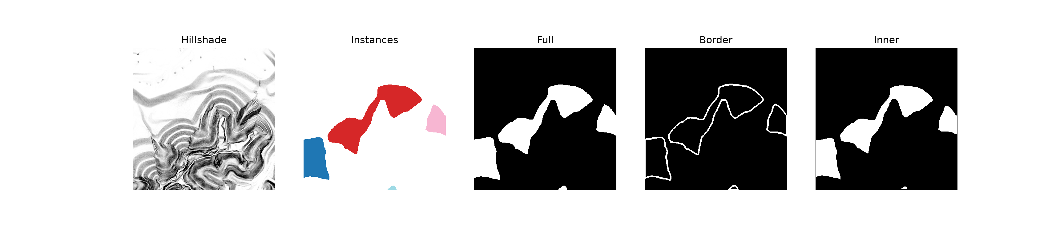
Since the derived masks depend on the full extent of each object, objects that are cut by the edge of a chip will have borders along the chip edge and inner segments that are shrunk away from it. An alternative is to derive the three masks from the instance raster for the entire area before chipping. Here, I derive the masks for each chip, which is simpler and allows the masks to be recalculated with different settings without recreating the chips.
22.3.3 DataSet
The DataSet below reads an image chip and its instance chip, derives the three masks, and applies Albumentations transforms. The three masks are passed to Albumentations as a list using the masks argument, along with the instance chip, so that the same geometric transformations are applied to all of them. I only use flips and 90-degree rotations. Brightness and contrast adjustments, which are common for photographs, are not appropriate here, since the LSP values have physical meanings. The image is returned as a float tensor with a shape of (C, H, W), and the masks are returned as a float tensor with a shape of (3, H, W), since each mask is a binary target for a separate output. The instance chip is also returned so that object-level assessment can be performed.
class UNetIDDataset(Dataset):
    def __init__(self, df, folder, split, transform=None):
        self.df = df
        self.folder = folder
        self.split = split
        self.transform = transform

    def __getitem__(self, idx):
        chpN = self.df.iloc[idx]["chpN"]
        with rio.open(f"{self.folder}{self.split}/images/{chpN}") as src:
            image = np.transpose(src.read().astype("float32"), (1, 2, 0))
        with rio.open(f"{self.folder}{self.split}/masks/{chpN}") as src:
            inst = src.read(1).astype("int32")
        masks = list(makeUNetIDMasks(inst))
        if self.transform is not None:
            out = self.transform(image=image, masks=masks + [inst])
            image, masks, inst = out["image"], out["masks"][:3], out["masks"][3]
        image = torch.from_numpy(np.ascontiguousarray(np.transpose(image, (2, 0, 1))))
        masks = torch.from_numpy(np.stack(masks).astype("float32"))
        inst = torch.from_numpy(np.ascontiguousarray(inst)).long()
        return image, masks, inst

    def __len__(self):
        return len(self.df)
trainTransform = A.Compose([A.HorizontalFlip(p=0.5), A.VerticalFlip(p=0.5), A.RandomRotate90(p=0.5)])
trainDS = UNetIDDataset(trainDF, folder, "train", trainTransform)
valDS = UNetIDDataset(valDF, folder, "val")
testDS = UNetIDDataset(testDF, folder, "test")
trainDL = DataLoader(trainDS, batch_size=4, shuffle=True, drop_last=True, num_workers=0)
valDL = DataLoader(valDS, batch_size=4, shuffle=False, num_workers=0)
testDL = DataLoader(testDS, batch_size=4, shuffle=False, num_workers=0)
image, masks, inst = next(iter(trainDL))
print(image.shape, masks.shape, inst.shape)torch.Size([4, 3, 512, 512]) torch.Size([4, 3, 512, 512]) torch.Size([4, 512, 512])22.4 Building UNet-ID
22.4.1 The UNet Branches
Each of the three branches is a UNet like the one built in Chapter 15. I define it using the double_conv() and up_conv() functions from that chapter. The branch returns the feature maps from its last decoder block as opposed to class logits, since these feature maps are passed to the fusion component of UNet-ID.
def double_conv(inChn, outChn):
    return nn.Sequential(
        nn.Conv2d(inChn, outChn, kernel_size=3, padding=1), nn.BatchNorm2d(outChn), nn.ReLU(inplace=True),
        nn.Conv2d(outChn, outChn, kernel_size=3, padding=1), nn.BatchNorm2d(outChn), nn.ReLU(inplace=True))

def up_conv(inChn, outChn):
    return nn.Sequential(nn.ConvTranspose2d(inChn, outChn, kernel_size=2, stride=2),
                         nn.BatchNorm2d(outChn), nn.ReLU(inplace=True))

class UNetBranch(nn.Module):
    def __init__(self, inChn=3, enChn=(16, 32, 64, 128), btnChn=256, dcChn=(128, 64, 32, 16)):
        super().__init__()
        self.enc = nn.ModuleList([double_conv(i, o) for i, o in zip((inChn,) + enChn[:-1], enChn)])
        self.btn = double_conv(enChn[-1], btnChn)
        upIn = (btnChn,) + dcChn[:-1]
        self.up = nn.ModuleList([up_conv(c, c) for c in upIn])
        self.dec = nn.ModuleList([double_conv(upIn[i] + enChn[::-1][i], dcChn[i]) for i in range(4)])
        self.outChn = dcChn[-1]

    def forward(self, x):
        skips = []
        for enc in self.enc:
            x = enc(x)
            skips.append(x)
            x = F.max_pool2d(x, 2)
        x = self.btn(x)
        for up, dec, skip in zip(self.up, self.dec, skips[::-1]):
            x = dec(torch.cat([up(x), skip], dim=1))
        return x
22.4.2 Fusion and Output Paths
UNet-ID instantiates three branches, one for each mask. In the forward() method, the input image is passed through all three branches, and their outputs are concatenated along the channel dimension. Each of the three output paths then receives the concatenated features and applies two 3x3 convolutional layers with 64 and 32 filters, each followed by batch normalization and a ReLU activation, and a final 1x1 convolution that returns a single logit per pixel. The model returns the three logit maps stacked along the channel dimension in the order full, border, inner. Since each mask is a separate binary prediction, a sigmoid, as opposed to a softmax, is applied to obtain probabilities, and the three probabilities do not need to sum to 1.
class UNetID(nn.Module):
    def __init__(self, inChn=3, enChn=(16, 32, 64, 128), btnChn=256, dcChn=(128, 64, 32, 16)):
        super().__init__()
        self.branches = nn.ModuleList([UNetBranch(inChn, enChn, btnChn, dcChn) for _ in range(3)])
        catChn = 3 * dcChn[-1]
        self.paths = nn.ModuleList([
            nn.Sequential(
                nn.Conv2d(catChn, 64, kernel_size=3, padding=1), nn.BatchNorm2d(64), nn.ReLU(inplace=True),
                nn.Conv2d(64, 32, kernel_size=3, padding=1), nn.BatchNorm2d(32), nn.ReLU(inplace=True),
                nn.Conv2d(32, 1, kernel_size=1))
            for _ in range(3)])

    def forward(self, x):
        feats = torch.cat([b(x) for b in self.branches], dim=1)
        return torch.cat([p(feats) for p in self.paths], dim=1)   # (N, 3, H, W): full, border, inner
model = UNetID(inChn=3)
x = torch.rand(2, 3, 512, 512)
print(model(x).shape)torch.Size([2, 3, 512, 512])summary(model, (2, 3, 512, 512), depth=2, device="cpu")====================================================================================================
Layer (type:depth-idx) Output Shape Param #
====================================================================================================
UNetID [2, 3, 512, 512] --
├─ModuleList: 1-1 -- --
│ └─UNetBranch: 2-1 [2, 16, 512, 512] 2,315,152
│ └─UNetBranch: 2-2 [2, 16, 512, 512] 2,315,152
│ └─UNetBranch: 2-3 [2, 16, 512, 512] 2,315,152
├─ModuleList: 1-2 -- --
│ └─Sequential: 2-4 [2, 1, 512, 512] 46,401
│ └─Sequential: 2-5 [2, 1, 512, 512] 46,401
│ └─Sequential: 2-6 [2, 1, 512, 512] 46,401
====================================================================================================
Total params: 7,084,659
Trainable params: 7,084,659
Non-trainable params: 0
Total mult-adds (Units.GIGABYTES): 182.77
====================================================================================================
Input size (MB): 6.29
Forward/backward pass size (MB): 7008.68
Params size (MB): 28.34
Estimated Total Size (MB): 7043.31
====================================================================================================Since UNet-ID contains three complete UNets, it has roughly three times as many parameters as a single UNet. An alternative design, which reduces the number of parameters, is to use a single shared encoder and decoder with three output paths.
22.5 Training with Lightning
22.5.1 Loss
Each of the three outputs is a binary segmentation, so each requires a binary loss. I combine binary cross entropy (calculated from logits for numerical stability, as discussed in Chapter 4) and Dice loss for each output and sum the losses for the three outputs using weights. The border and inner masks are thin or small regions that are highly imbalanced relative to the background, which is why the Dice component is useful. Increasing the weight for the border output can improve the separation of touching objects. Since the valley fill faces do not touch, I weight the three outputs equally.
class UNetIDLoss(nn.Module):
    def __init__(self, weights=(1.0, 1.0, 1.0), diceWght=1.0, smooth=1.0):
        super().__init__()
        self.weights = weights
        self.diceWght = diceWght
        self.smooth = smooth

    def _diceLoss(self, logits, target):
        probs = torch.sigmoid(logits)
        TP = (probs * target).sum()
        dice = (2*TP + self.smooth) / (probs.sum() + target.sum() + self.smooth)
        return 1 - dice

    def forward(self, logits, targets):              # both (N, 3, H, W)
        logits = logits.float()
        total = 0.0
        for k in range(3):
            l, t = logits[:, k], targets[:, k]
            total = total + self.weights[k] * (F.binary_cross_entropy_with_logits(l, t)
                                               + self.diceWght * self._diceLoss(l, t))
        return total
22.5.2 LightningModule
Since the DataSet returns three items (the image, the masks, and the instance chip) and the model returns three outputs, I define a LightningModule specifically for UNet-ID as opposed to using the LitSegmenter from Chapter 16. I log the binary F1-score for each of the three outputs separately. The validation F1-score for the full mask is used to select the best model. Since the separation of instances depends on the post-processing step, object-level assessment is performed after training, as described below.
class LitUNetID(L.LightningModule):
    def __init__(self, model, lr=1e-3, lossWeights=(1.0, 1.0, 1.0)):
        super().__init__()
        self.save_hyperparameters(ignore=["model"])
        self.model = model
        self.criterion = UNetIDLoss(weights=lossWeights)
        self.lr = lr
        self.names = ["full", "border", "inner"]
        self.train_f1 = nn.ModuleList([tm.F1Score(task="binary") for _ in range(3)])
        self.val_f1 = nn.ModuleList([tm.F1Score(task="binary") for _ in range(3)])

    def forward(self, x):
        return self.model(x)

    def _shared_step(self, batch, f1s, stage):
        x, masks, _ = batch
        logits = self(x)
        loss = self.criterion(logits, masks)
        self.log(f"{stage}_loss", loss, on_step=False, on_epoch=True, prog_bar=True)
        for k, name in enumerate(self.names):
            f1s[k].update(torch.sigmoid(logits[:, k].float()), masks[:, k].long())
            self.log(f"{stage}_f1_{name}", f1s[k], on_step=False, on_epoch=True,
                     prog_bar=(stage == "val" and name == "full"))
        return loss

    def training_step(self, batch, batch_idx):
        return self._shared_step(batch, self.train_f1, "train")

    def validation_step(self, batch, batch_idx):
        self._shared_step(batch, self.val_f1, "val")

    def predict_step(self, batch, batch_idx):
        return torch.sigmoid(self(batch[0]))

    def configure_optimizers(self):
        optimizer = torch.optim.AdamW(self.parameters(), lr=self.lr)
        scheduler = torch.optim.lr_scheduler.OneCycleLR(
            optimizer, max_lr=self.lr * 10, total_steps=self.trainer.estimated_stepping_batches)
        return {"optimizer": optimizer, "lr_scheduler": {"scheduler": scheduler, "interval": "step"}}
I train the model for 50 epochs with a mini-batch size of 4, using the AdamW optimizer with a one-cycle learning rate schedule with a maximum learning rate of 1e-3 and bfloat16 mixed precision. Since UNet-ID contains three UNets and the chips are 512x512 cells, a mini-batch size of 8 required nearly all of the memory on my 12 GB GPU and made training roughly eight times slower per chip, so I use a mini-batch size of 4. The checkpoint with the highest validation F1-score for the full mask is retained. After training, I save the state dictionary of the best model.
L.seed_everything(42)
litModel = LitUNetID(UNetID(inChn=3), lr=1e-4)
ckpt = ModelCheckpoint(dirpath="data/output/unetidVfill/", filename="best",
                       monitor="val_f1_full", mode="max")
trainer = L.Trainer(max_epochs=50, accelerator="gpu", devices=1, precision="bf16-mixed",
                    callbacks=[ckpt], logger=CSVLogger("data/output/", name="unetidVfill"))
trainer.fit(litModel, train_dataloaders=trainDL, val_dataloaders=valDL)

best = LitUNetID.load_from_checkpoint(ckpt.best_model_path, model=UNetID(inChn=3))
torch.save(best.model.state_dict(), "data/output/unetidVfill.pt")
Training took roughly 73 minutes. The highest validation F1-score for the full mask, 0.813, was obtained at epoch 41, so this checkpoint was saved. Below, I plot the training and validation losses and the validation F1-scores for the three masks. The validation metrics fluctuate during the early epochs, when the learning rate is high, and stabilize as the learning rate is reduced near the end of the one-cycle schedule. The training loss continues to decrease while the validation loss levels off after about 30 epochs, which suggests that additional epochs would not improve the model and that it is beginning to overfit the single training area. The full and inner masks are predicted with similar F1-scores of about 0.81, while the F1-score for the border mask is much lower, about 0.50. This is expected, since the borders are thin, so being off by even one or two cells along a boundary has a large impact on the F1-score.
resultsDF = pd.read_csv("data/models/unetidVfillLogs.csv")
trainRes = resultsDF.dropna(subset=["train_loss"])
valRes = resultsDF.dropna(subset=["val_loss"])

fig, axs = plt.subplots(1, 2, figsize=(12, 4))
axs[0].plot(trainRes["epoch"], trainRes["train_loss"], label="Training")
axs[0].plot(valRes["epoch"], valRes["val_loss"], label="Validation")
axs[0].set_title("Loss")
axs[0].legend()
for name in ["full", "border", "inner"]:
    axs[1].plot(valRes["epoch"], valRes[f"val_f1_{name}"], label=name.capitalize())
axs[1].set_title("Validation F1-score")
axs[1].legend()
for ax in axs:
    ax.set_xlabel("Epoch")
plt.show()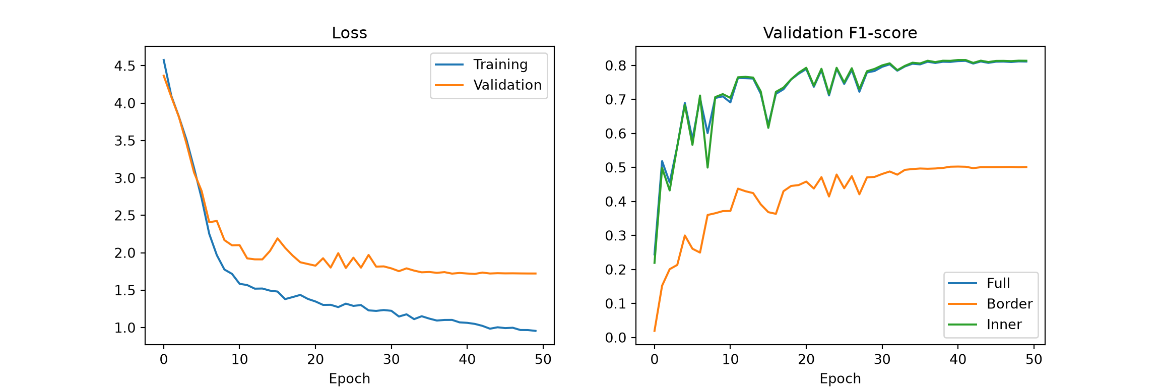
To use the trained model, I load the saved state dictionary into a new instance of UNet-ID.
model = UNetID(inChn=3)
model.load_state_dict(torch.load("data/models/unetidVfill.pt", map_location=device))
model = model.to(device).eval()
22.6 Separating Instances
After the three masks are predicted, individual objects are separated in a post-processing step. I use the following approach, which follows the logic of UNet-ID:
- Threshold the predicted probabilities for the three masks (e.g., at 0.5) to obtain binary masks.
- Remove the predicted borders from the predicted inner segments to make sure that neighboring inner segments are separated.
- Label each connected region of the resulting inner mask as a separate object using
scipy.ndimage.label(). These are the markers, or seeds, for the individual objects. Very small markers, which are often noise, are removed. - Grow the markers back to the full object extent using the watershed algorithm, which assigns each pixel of the predicted full mask to the nearest marker, using the predicted border probability as the “elevation” surface so that the boundaries between objects follow the predicted borders.
- Remove objects smaller than a minimum size. I use 200 cells (800 m2), the same minimum size used for the reference objects below.
The result is an instance raster grid in which each predicted object has a unique ID. Pixels that are in the full mask but cannot be reached from any marker remain unlabeled.
def removeSmall(inst, minPix):
    ids, counts = np.unique(inst, return_counts=True)
    small = ids[(counts < minPix) & (ids != 0)]
    return np.where(np.isin(inst, small), 0, inst)

def separateInstances(probs, thresh=0.5, minMarker=20, minObj=200):
    """probs: numpy array (3, H, W) of probabilities for full, border, inner."""
    full = probs[0] > thresh
    border = probs[1] > thresh
    inner = (probs[2] > thresh) & ~border & full
    markers = ndi.label(inner)[0]
    markers = removeSmall(markers, minMarker)
    predInst = watershed(probs[1], markers=markers, mask=full)
    return removeSmall(predInst, minObj)
22.7 Object-Level Assessment
Pixel-level metrics, such as the F1-score for the full mask, describe how well the object pixels were mapped, but they do not describe how well individual objects were separated. A model that maps every object pixel correctly but merges every pair of touching objects would have a high pixel-level F1-score but a poor count of objects. So, instance segmentation should also be assessed at the object level.
A common approach is to match predicted objects to reference objects using the intersection over union (IoU) of their masks. A predicted object that overlaps a reference object with an IoU greater than a threshold, commonly 0.5, is a true positive. Each reference object can be matched to at most one predicted object. Unmatched predicted objects are false positives, and unmatched reference objects are false negatives. Object-level precision, recall, and F1-score can then be calculated from these counts. With an IoU threshold of at least 0.5, each reference object can overlap at most one predicted object by more than this amount, so the matching is unambiguous. The function below implements this matching. Reference objects smaller than 200 cells, which are mostly slivers of valley fill faces cut by the chip edges, are removed before matching; the same rule is used in Chapter 23. In Chapter 23, we will also explore mean average precision (mAP), which summarizes performance across confidence thresholds and IoU thresholds.
def objectMetrics(refInst, predInst, iouThresh=0.5, minRef=200):
    refInst = removeSmall(refInst, minRef)
    refIDs = [i for i in np.unique(refInst) if i != 0]
    predIDs = [i for i in np.unique(predInst) if i != 0]
    matchedPred = set()
    TP = 0
    for r in refIDs:
        rMask = refInst == r
        cand = np.unique(predInst[rMask])
        for p in cand[cand != 0]:
            if p in matchedPred:
                continue
            pMask = predInst == p
            iou = (rMask & pMask).sum() / (rMask | pMask).sum()
            if iou > iouThresh:
                TP += 1
                matchedPred.add(p)
                break
    FP = len(predIDs) - TP
    FN = len(refIDs) - TP
    return {"TP": TP, "FP": FP, "FN": FN}

def summarizeCounts(totals):
    P = totals["TP"] / max(totals["TP"] + totals["FP"], 1)
    R = totals["TP"] / max(totals["TP"] + totals["FN"], 1)
    F1 = 2 * P * R / max(P + R, 1e-6)
    return {**totals, "Precision": round(P, 3), "Recall": round(R, 3), "F1": round(F1, 3)}
I predict the VA1 test chips in mini-batches, calculate the pixel-level F1-score for each of the three masks, and separate and assess the instances for each chip. The probabilities are retained for plotting.
testF1 = [tm.F1Score(task="binary") for _ in range(3)]
totals = {"TP": 0, "FP": 0, "FN": 0}
allProbs, allPredInst = [], []
with torch.no_grad():
    for image, masks, inst in testDL:
        probs = torch.sigmoid(model(image.to(device)).float()).cpu()
        for k in range(3):
            testF1[k].update(probs[:, k], masks[:, k].long())
        for p, ref in zip(probs.numpy(), inst.numpy()):
            predInst = separateInstances(p)
            m = objectMetrics(ref, predInst)
            for k in totals:
                totals[k] += m[k]
            allProbs.append(p)
            allPredInst.append(predInst)

print({n: round(float(f.compute()), 3) for n, f in zip(["full", "border", "inner"], testF1)})
{'full': 0.658, 'border': 0.397, 'inner': 0.658}summarizeCounts(totals){'TP': 82, 'FP': 93, 'FN': 103, 'Precision': 0.469, 'Recall': 0.443, 'F1': 0.456}The pixel-level F1-scores for the VA1 test chips (0.658 for the full and inner masks and 0.397 for the border mask) are lower than those for the KY2 validation chips. As in Chapter 23, this suggests that the model, trained using a single study area, does not generalize perfectly to new areas. At the object level, 82 of the 185 reference valley fill faces were matched with an IoU greater than 0.5, for a precision of 0.469, a recall of 0.443, and an F1-score of 0.456. As with Mask R-CNN, these chip-based metrics are pessimistic: the test chips are a grid, so many valley fill faces are cut by the chip edges, and partial objects are harder to detect and match. A predicted object that covers only part of a reference object, or that merges a valley fill face with adjacent mined terrain, will also fail to meet the IoU threshold even if the valley fill was detected.
To visualize the results, I plot the hillshade, the reference instances, the predicted probabilities for the three masks, and the separated instances for several test chips.
showIdx = testDF.index[testDF["nInst"] >= 2][[0, 5, 10, 15]]
fig, axs = plt.subplots(4, 6, figsize=(18, 12))
for row, i in enumerate(showIdx):
    image, masks, inst = testDS[i]
    hs = image[2].numpy()
    axs[row, 0].imshow(hs, cmap="gray", vmin=np.quantile(hs, 0.01), vmax=np.quantile(hs, 0.99))
    axs[row, 1].imshow(np.ma.masked_equal(inst.numpy(), 0) % 20, cmap="tab20", interpolation="nearest")
    for k in range(3):
        axs[row, 2 + k].imshow(allProbs[i][k], cmap="viridis", vmin=0, vmax=1)
    axs[row, 5].imshow(np.ma.masked_equal(allPredInst[i], 0) % 20, cmap="tab20", interpolation="nearest")
for ax, t in zip(axs[0], ["Hillshade", "Reference", "Full", "Border", "Inner", "Predicted"]):
    ax.set_title(t)
for ax in axs.flat:
    ax.axis("off")
plt.show()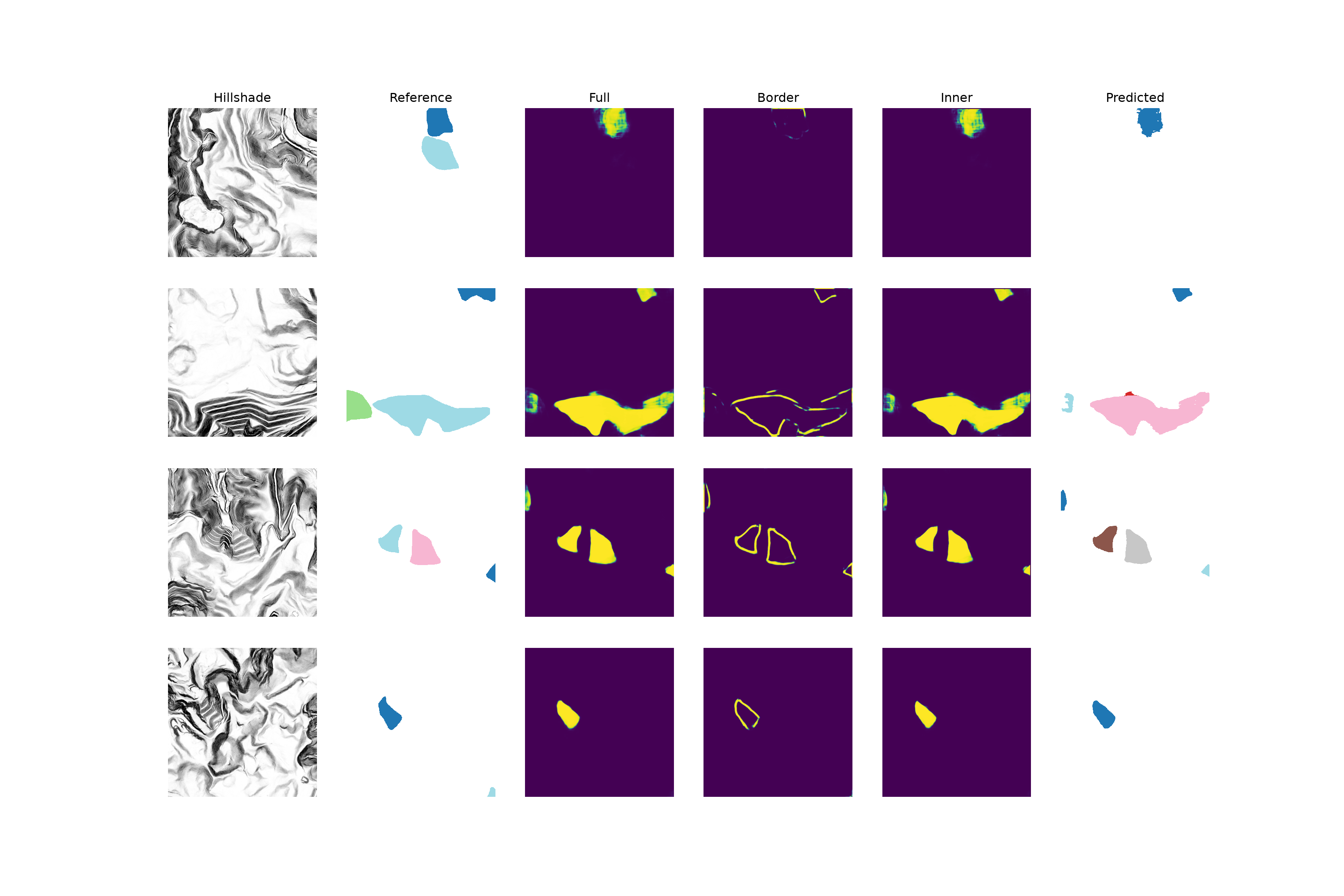
For most of the valley fill faces shown, the full and inner probabilities are high within the object and low elsewhere, and the predicted borders outline each valley fill face, so the separated instances closely match the reference objects. Errors include a missed valley fill face, a large valley fill face accompanied by a small spurious fragment, and objects cut by the chip edges that are only partially predicted. The border predictions within the large valley fill face in the second row also follow some of the benches that run across the fill; since the inner segment remains connected, the face is still recovered as a single object.
22.8 Predicting to Geospatial Data
To produce a map, UNet-ID is applied to an entire area using the methods from Chapter 19, and the instances are separated for the entire area as opposed to separately for each chip. This avoids splitting objects along the chip edges. The predictDTM() function below performs the following steps for a rectangular area within a DTM:
- The DTM is read for the area plus a 64-cell buffer, and the LSPs are calculated using
lspModulewith the same settings used to create the chips. The buffer is then removed, which avoids the edge effects described above. - The LSP stack is processed as overlapping 512x512 chips. With a
strideof 384, adjacent chips overlap by 128 cells. Predictions near the edges of the chips are less reliable, since less spatial context is available, so only the central portion of each chip’s predicted probabilities is written to the output, except along the edges of the area. This is the same cropping and mosaicking approach used in Chapter 19. - The instances are separated using the probabilities for the entire area.
lspM = lspModule(cell_size=2.0, spat_dim=640, inner_radius=1, outer_radius=5,
                 hs_radius=25, smooth_radius=6).to(device).eval()

def predictDTM(model, lspM, dtmPath, bounds, chipSize=512, stride=384, pad=64):
    with rio.open(dtmPath) as src:
        win = from_bounds(*bounds, transform=src.transform).round_offsets().round_lengths()
        r0, c0, H, W = int(win.row_off), int(win.col_off), int(win.height), int(win.width)
        dtm = src.read(1, window=((r0 - pad, r0 + H + pad), (c0 - pad, c0 + W + pad)))
        areaTransform = src.window_transform(win)

    with torch.no_grad():
        lsps = lspM(torch.from_numpy(dtm).float()[None, None].to(device))
    lsps = lsps[0, [0, 1, 3], pad:-pad, pad:-pad]       # tpiHS, slp, hillshade

    def starts(n):
        s = list(range(0, n - chipSize + 1, stride))
        return s if s[-1] == n - chipSize else s + [n - chipSize]

    margin = (chipSize - stride) // 2
    probs = np.zeros((3, H, W), dtype="float32")
    rowStarts, colStarts = starts(H), starts(W)
    for r in rowStarts:
        for c in colStarts:
            with torch.no_grad():
                p = torch.sigmoid(model(lsps[None, :, r:r + chipSize, c:c + chipSize]).float())[0]
            p = p.cpu().numpy()
            # Central portion of the chip (full extent at the area's edges)
            y0 = 0 if r == rowStarts[0] else margin
            y1 = chipSize if r == rowStarts[-1] else chipSize - margin
            x0 = 0 if c == colStarts[0] else margin
            x1 = chipSize if c == colStarts[-1] else chipSize - margin
            probs[:, r + y0:r + y1, c + x0:c + x1] = p[:, y0:y1, x0:x1]
    return probs, lsps[2].cpu().numpy(), areaTransform
I apply the function to the same 4x4 km area within the VA1 test area that is mapped using Mask R-CNN in Chapter 23. The DTM and the reference polygons are in different coordinate reference systems, so the polygons are projected to match the DTM. To assess the results for the area, I rasterize the reference polygons that intersect the area to an instance raster aligned with the predictions using the makeInstanceRaster() function defined above and calculate the object-level metrics. Unlike the chip-based assessment, few objects are cut by the edges of the area.
# Set these to the location of the uncompressed vfillDL folder on your machine.
dtmPath = "data/files/vfillDL/dems/va1_dem.tif"
with rio.open(dtmPath) as src:
    dtmCRS = src.crs
refGDF = gpd.read_file("data/files/vfillDL/vectors/testingVA1.shp").to_crs(dtmCRS)

areaBounds = (348800, 4100100, 352800, 4104100)   # xmin, ymin, xmax, ymax
probs, hillshade, areaTransform = predictDTM(model, lspM, dtmPath, areaBounds)
predInst = separateInstances(probs)

refArea = refGDF[refGDF.intersects(box(*areaBounds))]
refInst = makeInstanceRaster(refArea, predInst.shape, areaTransform)
summarizeCounts(objectMetrics(refInst, predInst))
{'TP': 17, 'FP': 6, 'FN': 3, 'Precision': 0.739, 'Recall': 0.85, 'F1': 0.791}The predicted instance raster can be converted to polygons for use in a GIS using rasterio.features.shapes(), which returns the geometry of each connected region of equal value. Providing the transform for the area returns the polygons in map coordinates.
def instancesToPolygons(predInst, transform, crs):
    geoms = [(shape(g), int(v)) for g, v in features.shapes(predInst.astype("int32"),
                                                            mask=predInst > 0, transform=transform)]
    gdf = gpd.GeoDataFrame({"id": [v for _, v in geoms]}, geometry=[g for g, _ in geoms], crs=crs)
    return gdf.dissolve(by="id").reset_index()

predGDF = instancesToPolygons(predInst, areaTransform, dtmCRS)
print(f"Predicted: {len(predGDF)}, Reference: {len(refArea)}")
Predicted: 23, Reference: 20fig, axs = plt.subplots(1, 2, figsize=(14, 7))
extent = [areaBounds[0], areaBounds[2], areaBounds[1], areaBounds[3]]
for ax, gdf, color, title in zip(axs, [refArea, predGDF], ["yellow", "cyan"],
["Reference", "UNet-ID"]):
ax.imshow(hillshade, cmap="gray", extent=extent, vmin=np.quantile(hillshade, 0.01),
vmax=np.quantile(hillshade, 0.99))
gdf.boundary.plot(ax=ax, color=color, linewidth=1)
ax.set_xlim(extent[0], extent[1])
ax.set_ylim(extent[2], extent[3])
ax.set_title(title)
ax.axis("off")
plt.show()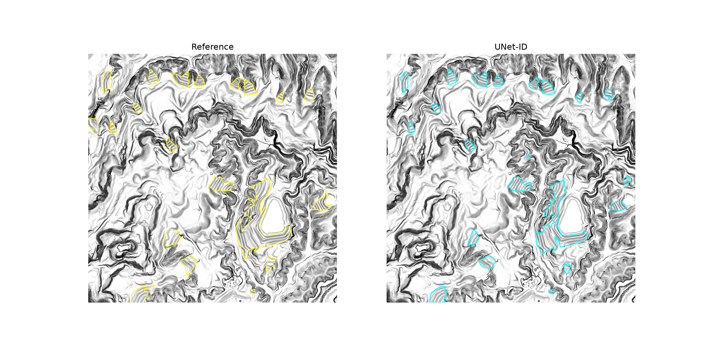
For this area, 23 valley fill faces were predicted, compared to 20 reference valley fill faces that intersect the area. Of these, 17 were matched with an IoU greater than 0.5, giving a precision of 0.739, a recall of 0.850, and an F1-score of 0.791. These results are much better than those for the test chips, since few valley fill faces are cut by the edges of the area. Most of the valley fill faces are mapped with boundaries that closely follow the reference boundaries. As with Mask R-CNN, most of the errors occur within the large, complex mined area in the center, where some predictions only partially correspond to the reference polygons, and a few small false positives occur elsewhere. Interestingly, Mask R-CNN produced exactly the same counts for this area, so the two approaches performed similarly here; Chapter 23 compares them in more detail.
22.9 Concluding Remarks
In this chapter, we built UNet-ID, a segmentation-based instance segmentation architecture, from scratch. By predicting object borders and inner segments in addition to the full object extent, the model provides the information needed to separate touching objects in a post-processing step. This approach builds on the semantic segmentation architectures and training processes explored in the prior chapters, and it can be adapted to other objects that are difficult to separate, such as buildings and tree crowns. In the next chapter, we will explore a detection-based alternative, Mask R-CNN, which predicts the instances directly, using the same valley fill data.
22.10 Questions
- Explain the difference between semantic segmentation and instance segmentation. Give two geospatial applications for which instance segmentation is required.
- Explain the difference between detection-based and segmentation-based approaches to instance segmentation.
- Describe the three masks predicted by UNet-ID and how each is derived from an instance raster using erosion and dilation. Why must the operations be applied separately to each object?
- Why does predicting object borders and inner segments allow touching objects to be separated?
- Describe the structure of the UNet-ID architecture, including the three branches and the fusion and output paths. Why is a sigmoid, as opposed to a softmax, applied to the outputs?
- Explain the post-processing steps used to separate the predicted objects into instances, including the roles of the markers and the watershed algorithm.
- Why are pixel-level metrics insufficient for assessing instance segmentation? Explain how predicted and reference objects are matched using intersection over union (IoU) to calculate object-level precision and recall.
- How should the number of pixels used to define the inner segments and borders be selected for data with a different spatial resolution or objects of a different size than those used in the original paper?