import torch
import torch.nn as nn
import torch.nn.functional as F
from torchinfo import summary

device = torch.device("cuda:0" if torch.cuda.is_available() else "cpu")18 UNet Modules
18.1 Introduction
In Chapter 15, we built a UNet from scratch, and in Chapter 17, we replaced its encoder with pre-trained CNN architectures. Another way to potentially improve a UNet is to add modules, or small sub-networks, at specific locations in the architecture. Many architecture modifications proposed in the literature are not entirely new architectures but rather a standard architecture, such as UNet, with one or more modules added. Examples include residual connections, which are central to ResNet; squeeze-and-excitation modules, which recalibrate the importance of feature maps; attention mechanisms along the skip connections, which suppress irrelevant features passed from the encoder to the decoder; atrous spatial pyramid pooling, which captures context at multiple spatial scales and is central to DeepLabv3+; and deep supervision, which provides additional training signals to the decoder.
In this chapter, we build each of these modules and then combine them into a single, customizable UNet architecture in which each module can be turned on or off using an argument. This makes it easy to experiment with different configurations and to design experiments that assess the impact of each module. The architecture mirrors the defineUNet() function in our geodl R package, which is discussed in our Geospatial Supervised Learning using R text, and the defineCUNet() class in our terrainseg Python package. So, if you have used either of those packages, the options will be familiar. The architecture has the following options:
- Activation function: ReLU, leaky ReLU, Swish, or GELU, as discussed in Chapter 7.
- Residual connections within the double convolution blocks in the encoder, decoder, and bottleneck.
- Squeeze-and-excitation (SE) modules applied to the output of each encoder block.
- Attention gates along the skip connections.
- Convolutional block attention modules (CBAM) along the skip connections.
- An atrous spatial pyramid pooling (ASPP) module as the bottleneck.
- Deep supervision, in which predictions are generated at each decoder resolution.
Similar to Chapter 15, the focus of this chapter is on defining the architecture. We will check each module using random data of the correct shape and summarize the architectures using torchinfo. At the end of the chapter, I show how to train the customizable UNet using PyTorch Lightning, including how to handle the multiple outputs produced when deep supervision is used.
18.2 Building Blocks
18.2.1 Activation Functions
To allow the activation function to be selected by the user, I define a helper function that returns the requested activation as an nn.Module. This is the same approach demonstrated in Chapter 7. A new activation layer is created each time the function is called, since the same layer object should not be reused in multiple locations within nn.Sequential().
def makeAct(actFunc="relu", negative_slope=0.01):
    actFunc = actFunc.lower()
    if actFunc == "lrelu":
        return nn.LeakyReLU(negative_slope=negative_slope, inplace=True)
    if actFunc == "swish":
        return nn.SiLU(inplace=True)
    if actFunc == "gelu":
        return nn.GELU()
    if actFunc == "relu":
        return nn.ReLU(inplace=True)
    raise ValueError("actFunc must be 'relu', 'lrelu', 'swish', or 'gelu'")
18.2.2 Double Convolution Blocks
The standard building block of UNet is the double convolution block, which we defined as a function in Chapter 15. Here, I define it as an nn.Module subclass that accepts the activation function as an argument.
class DoubleConvBlk(nn.Module):
    def __init__(self, inChn, outChn, actFunc="relu", negative_slope=0.01):
        super().__init__()
        self.block = nn.Sequential(
            nn.Conv2d(inChn, outChn, kernel_size=3, stride=1, padding=1),
            nn.BatchNorm2d(outChn),
            makeAct(actFunc, negative_slope),
            nn.Conv2d(outChn, outChn, kernel_size=3, stride=1, padding=1),
            nn.BatchNorm2d(outChn),
            makeAct(actFunc, negative_slope),
        )

    def forward(self, x):
        return self.block(x)
18.3 Residual Connections
Residual connections, introduced with the ResNet architecture (He et al., 2016), add the input of a block to its output. Instead of learning a complete transformation of its input, \(H(x)\), the block learns a residual, \(F(x) = H(x) - x\), and its output is \(F(x) + x\). If the best transformation is close to the identity, the block only needs to learn small adjustments. More importantly, the addition provides a direct path for the gradients to flow backward through the network during backpropagation, which reduces the vanishing gradient problem and allows much deeper networks to be trained.
He, K., Zhang, X., Ren, S. and Sun, J., 2016. “Deep residual learning for image recognition.” In Proceedings of the IEEE Conference on Computer Vision and Pattern Recognition (pp. 770-778).
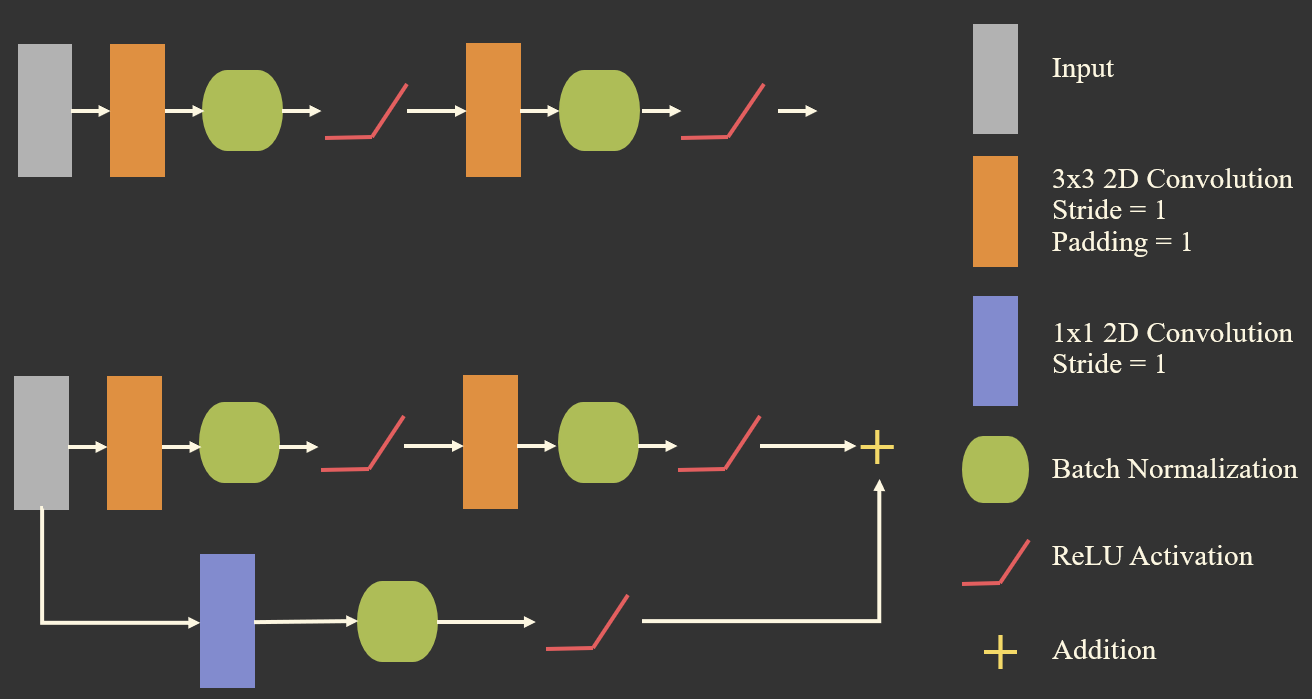
In a double convolution block, the number of channels generally changes, so the input cannot be added to the output directly since their shapes differ. Instead, the input is passed through a 1x1 convolution that projects it to the correct number of channels. This projection is sometimes called a shortcut or skip path. Following the design of ResNet, the second convolution in the residual path is followed by batch normalization but not an activation function; the activation is applied after the addition.
A standard double convolution block and a double convolution block with a residual connection are compared in Figure 18.1.
class FeatReduce(nn.Module):
    """1x1 convolution, optionally followed by batch normalization and an activation."""
    def __init__(self, inChn, outChn, actFunc="relu", doBnAct=True, negative_slope=0.01):
        super().__init__()
        self.conv = nn.Conv2d(inChn, outChn, kernel_size=1, stride=1, padding=0)
        self.bnAct = nn.Sequential(nn.BatchNorm2d(outChn), makeAct(actFunc, negative_slope)) if doBnAct else nn.Identity()

    def forward(self, x):
        return self.bnAct(self.conv(x))


class DoubleConvBlkR(nn.Module):
    """Residual double convolution: (conv-BN-act-conv-BN) + 1x1 projection, then activation."""
    def __init__(self, inChn, outChn, actFunc="relu", negative_slope=0.01):
        super().__init__()
        self.res = nn.Sequential(
            nn.Conv2d(inChn, outChn, kernel_size=3, stride=1, padding=1),
            nn.BatchNorm2d(outChn),
            makeAct(actFunc, negative_slope),
            nn.Conv2d(outChn, outChn, kernel_size=3, stride=1, padding=1),
            nn.BatchNorm2d(outChn),
        )
        self.skip = FeatReduce(inChn, outChn, actFunc, doBnAct=False)
        self.finalAct = makeAct(actFunc, negative_slope)

    def forward(self, x):
        return self.finalAct(self.res(x) + self.skip(x))
x = torch.rand(4, 32, 64, 64)
print(DoubleConvBlkR(32, 64, actFunc="gelu")(x).shape) # torch.Size([4, 64, 64, 64])18.4 Squeeze-and-Excitation Modules
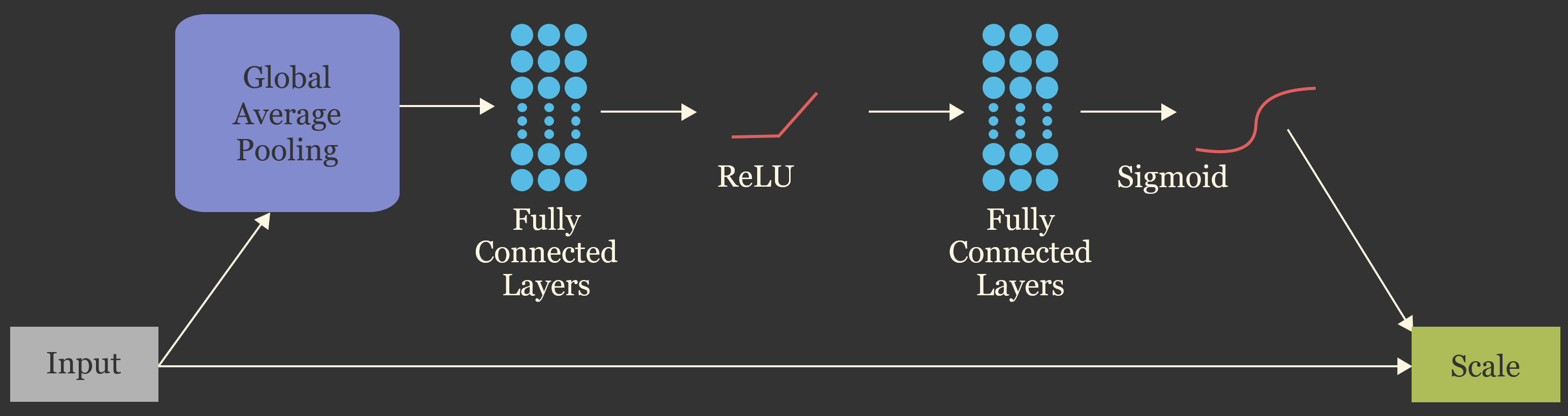
A convolutional layer generates many feature maps, but not all of them are equally useful for a particular input. Squeeze-and-excitation (SE) modules (Hu et al., 2018) learn to reweight the feature maps, emphasizing informative channels and suppressing less useful ones. This is a form of channel attention. The module consists of three steps:
- Squeeze: global average pooling summarizes each feature map as a single value, producing a vector with one value per channel. This captures the global context of the input.
- Excitation: the vector is passed through two fully connected layers. The first reduces the number of values by a factor called the reduction ratio (e.g., 8 or 16), followed by a ReLU activation, and the second restores the original number of values, followed by a sigmoid activation. The result is a weight between 0 and 1 for each channel. The reduction forces the module to learn relationships between the channels while limiting the number of added parameters.
- Scale: each feature map is multiplied by its weight.
These steps are conceptualized in Figure 18.2.
Hu, J., Shen, L. and Sun, G., 2018. “Squeeze-and-excitation networks.” In Proceedings of the IEEE Conference on Computer Vision and Pattern Recognition (pp. 7132-7141).
In our architecture, SE modules are applied to the output of each encoder block, before max pooling. As a result, they influence both the features passed to the next encoder block and the features passed to the decoder via the skip connection. SE modules add relatively few parameters and computations.
class SEModule(nn.Module):
    def __init__(self, inChn, ratio=8):
        super().__init__()
        hidden = max(1, inChn // ratio)
        self.pool = nn.AdaptiveAvgPool2d(1)
        self.fc = nn.Sequential(
            nn.Linear(inChn, hidden, bias=False),
            nn.ReLU(inplace=True),
            nn.Linear(hidden, inChn),
            nn.Sigmoid(),
        )

    def forward(self, x):
        b, c, _, _ = x.shape
        w = self.fc(self.pool(x).view(b, c)).view(b, c, 1, 1)  # squeeze and excitation
        return x * w                                            # scale
x = torch.rand(4, 64, 64, 64)
print(SEModule(64, ratio=8)(x).shape) # same shape as the input18.5 Attention Gates
In a UNet, the skip connections pass all of the feature maps from each encoder block to the decoder. However, the encoder features at high resolution, especially those from the first blocks, capture low-level patterns, such as edges, across the entire image, much of which may be irrelevant to the classes of interest. Attention gates (Oktay et al., 2018) filter the skip connection features using information from the decoder, which has a coarser but more semantically meaningful representation of the image. The result is a spatial attention map with values between 0 and 1 that is multiplied by the skip connection features, suppressing regions that are unlikely to be relevant.
Oktay, O., Schlemper, J., Folgoc, L.L., Lee, M., Heinrich, M., Misawa, K., Mori, K., McDonagh, S., Hammerla, N.Y., Kainz, B. and Glocker, B., 2018. “Attention U-Net: Learning where to look for the pancreas.” arXiv preprint arXiv:1804.03999.
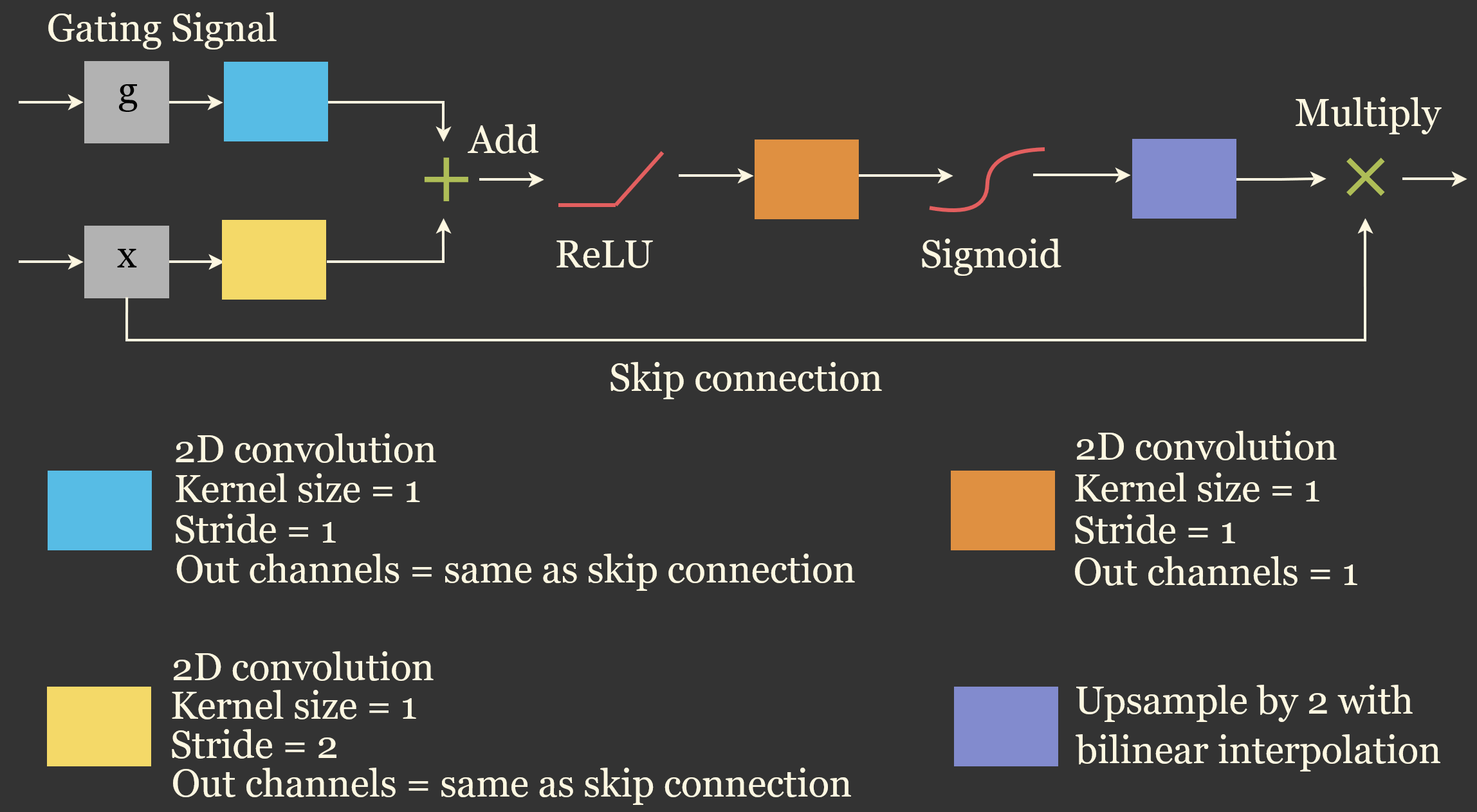
The attention gate accepts two inputs: the skip connection features from the encoder (\(x\)) and a gating signal (\(g\)), which is the output of the decoder block (or the bottleneck) at the next coarser resolution. The gate works as follows:
- The gating signal is passed through a 1x1 convolution that changes its number of channels to match the skip features.
- The skip features are passed through a 1x1 convolution with a stride of 2, which reduces their spatial dimensions by half so that they match the gating signal.
- The two results are added and passed through a ReLU activation. Regions where both the encoder and decoder features are strongly activated produce large values.
- A 1x1 convolution reduces the result to a single channel, and a sigmoid activation converts it to values between 0 and 1. This is the attention map.
- The attention map is upsampled by a factor of 2 to match the spatial dimensions of the skip features, and the skip features are multiplied by it.
Because the skip features are filtered before being concatenated with the decoder features, this is often called additive attention. The attention gate is conceptualized in Figure 18.3.
class AttnBlk(nn.Module):
    def __init__(self, xChn, gChn):
        super().__init__()
        self.W_gate = nn.Sequential(nn.Conv2d(gChn, xChn, kernel_size=1), nn.BatchNorm2d(xChn))
        self.W_x = nn.Sequential(nn.Conv2d(xChn, xChn, kernel_size=1, stride=2), nn.BatchNorm2d(xChn))
        self.psi = nn.Sequential(nn.Conv2d(xChn, 1, kernel_size=1), nn.BatchNorm2d(1), nn.Sigmoid())

    def forward(self, x, g):
        a = F.relu(self.W_gate(g) + self.W_x(x))
        a = self.psi(a)                                        # (N, 1, H/2, W/2)
        a = F.interpolate(a, scale_factor=2, mode="bilinear", align_corners=False)
        return x * a
x = torch.rand(4, 64, 64, 64) # skip features from the encoder
g = torch.rand(4, 128, 32, 32) # gating signal from the decoder at half the resolution
print(AttnBlk(64, 128)(x, g).shape) # torch.Size([4, 64, 64, 64])18.6 Convolutional Block Attention Module (CBAM)
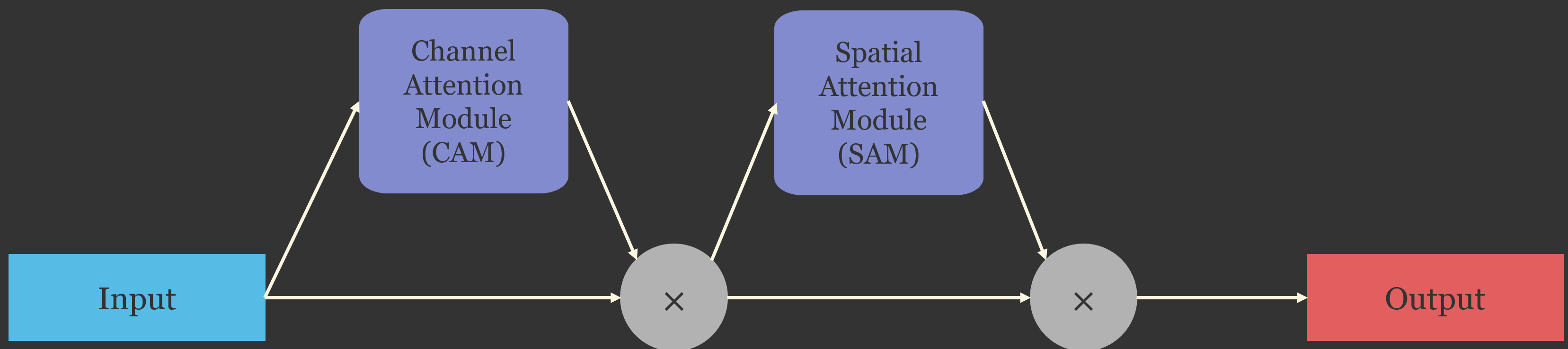
The convolutional block attention module (CBAM) (Woo et al., 2018) combines channel attention and spatial attention in sequence. Unlike the attention gate, it does not use a gating signal from the decoder; it recalibrates a set of features using only the features themselves.
Woo, S., Park, J., Lee, J.Y. and Kweon, I.S., 2018. “CBAM: Convolutional block attention module.” In Proceedings of the European Conference on Computer Vision (ECCV) (pp. 3-19).
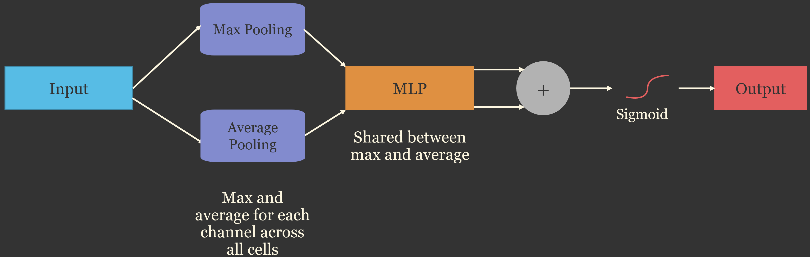
- Channel attention is similar to an SE module, except that both global average pooling and global max pooling are used to summarize each channel. Both summaries are passed through the same small network (a shared multilayer perceptron), and the results are added and passed through a sigmoid activation to obtain a weight for each channel.
- Spatial attention summarizes the channel-weighted features at each pixel location by taking the mean and maximum across all channels, producing two maps. These are concatenated and passed through a convolution with a large kernel (e.g., 7x7), followed by a sigmoid activation, to obtain a weight for each pixel location.
The overall structure of CBAM is shown in Figure 18.4, and its channel and spatial attention components are shown in Figure 18.5 and Figure 18.6, respectively.

In our architecture, CBAM modules are applied to the encoder features along each skip connection before they are concatenated with the decoder features. Since CBAM performs both channel and spatial recalibration, it overlaps with the SE modules and the attention gates. Following the design of geodl, when CBAM is used, the SE modules and attention gates are disabled.
class CBAMChannelAttn(nn.Module):
    def __init__(self, inChn, ratio=8):
        super().__init__()
        hidden = max(1, inChn // ratio)
        self.mlp = nn.Sequential(
            nn.Linear(inChn, hidden, bias=False),
            nn.ReLU(inplace=True),
            nn.Linear(hidden, inChn, bias=False),
        )

    def forward(self, x):
        b, c, _, _ = x.shape
        avg = self.mlp(F.adaptive_avg_pool2d(x, 1).view(b, c))
        mx = self.mlp(F.adaptive_max_pool2d(x, 1).view(b, c))
        return x * torch.sigmoid(avg + mx).view(b, c, 1, 1)


class CBAMSpatialAttn(nn.Module):
    def __init__(self, kernelSize=7):
        super().__init__()
        self.conv = nn.Sequential(
            nn.Conv2d(2, 1, kernel_size=kernelSize, padding=kernelSize // 2, bias=False),
            nn.BatchNorm2d(1),
            nn.Sigmoid(),
        )

    def forward(self, x):
        avgMap = torch.mean(x, dim=1, keepdim=True)
        maxMap = torch.amax(x, dim=1, keepdim=True)
        return x * self.conv(torch.cat([avgMap, maxMap], dim=1))


class CBAMBlk(nn.Module):
    def __init__(self, inChn, ratio=8, kernelSize=7):
        super().__init__()
        self.chanAttn = CBAMChannelAttn(inChn, ratio)
        self.spatAttn = CBAMSpatialAttn(kernelSize)

    def forward(self, x):
        return self.spatAttn(self.chanAttn(x))
x = torch.rand(4, 64, 64, 64)
print(CBAMBlk(64)(x).shape) # same shape as the input18.7 Atrous Spatial Pyramid Pooling (ASPP)
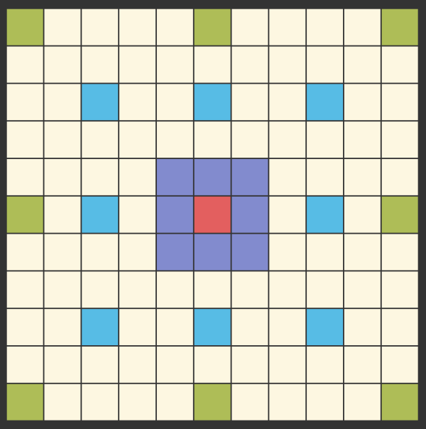
Many geospatial features can only be correctly identified using context over a broad area. Atrous (or dilated) convolution inserts gaps between the kernel weights so that the kernel covers a larger area without adding parameters or reducing the spatial resolution. A 3x3 kernel with a dilation rate of 6, for example, samples a 13x13 window. Atrous spatial pyramid pooling (ASPP), which is central to the DeepLab family of architectures (Chen et al., 2017, 2018), applies several atrous convolutions with different dilation rates in parallel, along with a 1x1 convolution and an image-level pooling branch, and concatenates the results. This captures context at multiple spatial scales simultaneously.
Atrous convolution is conceptualized in Figure 18.7, which shows the cells sampled by a 3x3 kernel centered on the same cell with three different dilation rates.
Chen, L.C., Papandreou, G., Schroff, F. and Adam, H., 2017. “Rethinking atrous convolution for semantic image segmentation.” arXiv preprint arXiv:1706.05587.
Chen, L.C., Zhu, Y., Papandreou, G., Schroff, F. and Adam, H., 2018. “Encoder-decoder with atrous separable convolution for semantic image segmentation.” In Proceedings of the European Conference on Computer Vision (ECCV) (pp. 801-818).
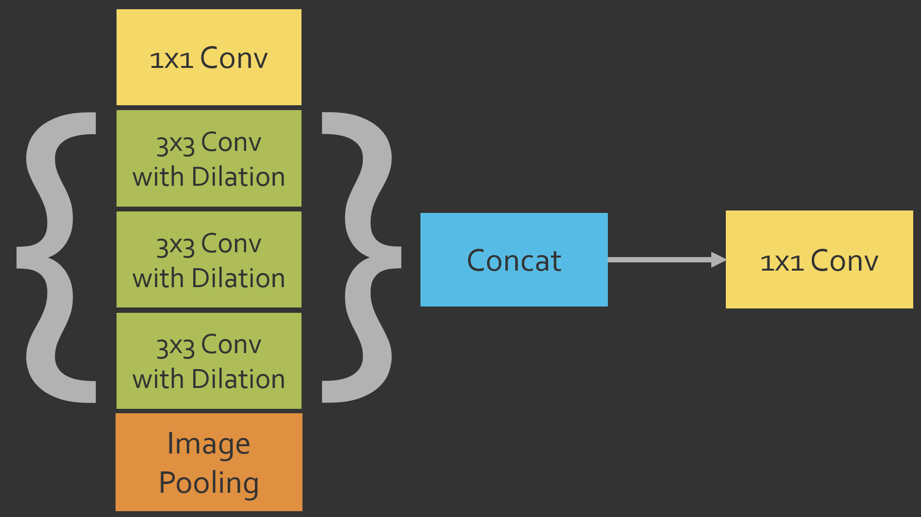
Our ASPP module, which replaces the double convolution block in the bottleneck, has five parallel branches:
- A 1x1 convolution.
- Three 3x3 atrous convolutions with different dilation rates (6, 12, and 18 by default). The padding is set equal to the dilation rate so that the spatial dimensions are maintained.
- An image pooling branch, which averages each input channel over the entire image and broadcasts the result back to the original spatial dimensions, providing global context.
The outputs are concatenated along the channel dimension and reduced to the desired number of output channels using a 1x1 convolution. A residual version adds a 1x1 projection of the input to the result before the final activation. The ASPP module is conceptualized in Figure 18.8.
When selecting dilation rates, keep in mind that the ASPP module operates on the bottleneck, which has a spatial resolution 1/16 of the input. For a 256x256 input chip, the bottleneck is 16x16, so a dilation rate of 18 samples locations that fall mostly in the zero-padding beyond the edges of the feature maps. The default rates were designed for larger feature maps. For small chips, smaller dilation rates, such as (2, 4, 6), may be more appropriate.
class AsppComp(nn.Module):
    def __init__(self, inChn, outChn, dilation, actFunc="relu", negative_slope=0.01):
        super().__init__()
        self.aspp = nn.Sequential(
            nn.Conv2d(inChn, outChn, kernel_size=3, stride=1, padding=dilation, dilation=dilation),
            nn.BatchNorm2d(outChn),
            makeAct(actFunc, negative_slope),
        )

    def forward(self, x):
        return self.aspp(x)


class GlobalAvgPool2d(nn.Module):
    def forward(self, x):
        h, w = x.shape[2:]
        return F.interpolate(F.adaptive_avg_pool2d(x, 1), size=(h, w), mode="bilinear", align_corners=False)


class AsppBlk(nn.Module):
    def __init__(self, inChn, outChn, dilChn=(256, 256, 256, 256), dilRates=(6, 12, 18),
                 actFunc="relu", useRes=False, negative_slope=0.01):
        super().__init__()
        self.useRes = useRes
        self.a1 = FeatReduce(inChn, dilChn[0], actFunc, negative_slope=negative_slope)
        self.a2 = AsppComp(inChn, dilChn[1], dilRates[0], actFunc, negative_slope)
        self.a3 = AsppComp(inChn, dilChn[2], dilRates[1], actFunc, negative_slope)
        self.a4 = AsppComp(inChn, dilChn[3], dilRates[2], actFunc, negative_slope)
        self.a5 = GlobalAvgPool2d()
        self.conv1x1 = FeatReduce(sum(dilChn) + inChn, outChn, actFunc, negative_slope=negative_slope)
        if useRes:
            self.skip = FeatReduce(inChn, outChn, actFunc, doBnAct=False)
            self.finalAct = makeAct(actFunc, negative_slope)

    def forward(self, x):
        out = torch.cat([self.a1(x), self.a2(x), self.a3(x), self.a4(x), self.a5(x)], dim=1)
        out = self.conv1x1(out)
        if self.useRes:
            out = self.finalAct(out + self.skip(x))
        return out
x = torch.rand(4, 128, 16, 16)
print(AsppBlk(128, 256, dilRates=(2, 4, 6))(x).shape) # torch.Size([4, 256, 16, 16])18.8 Deep Supervision
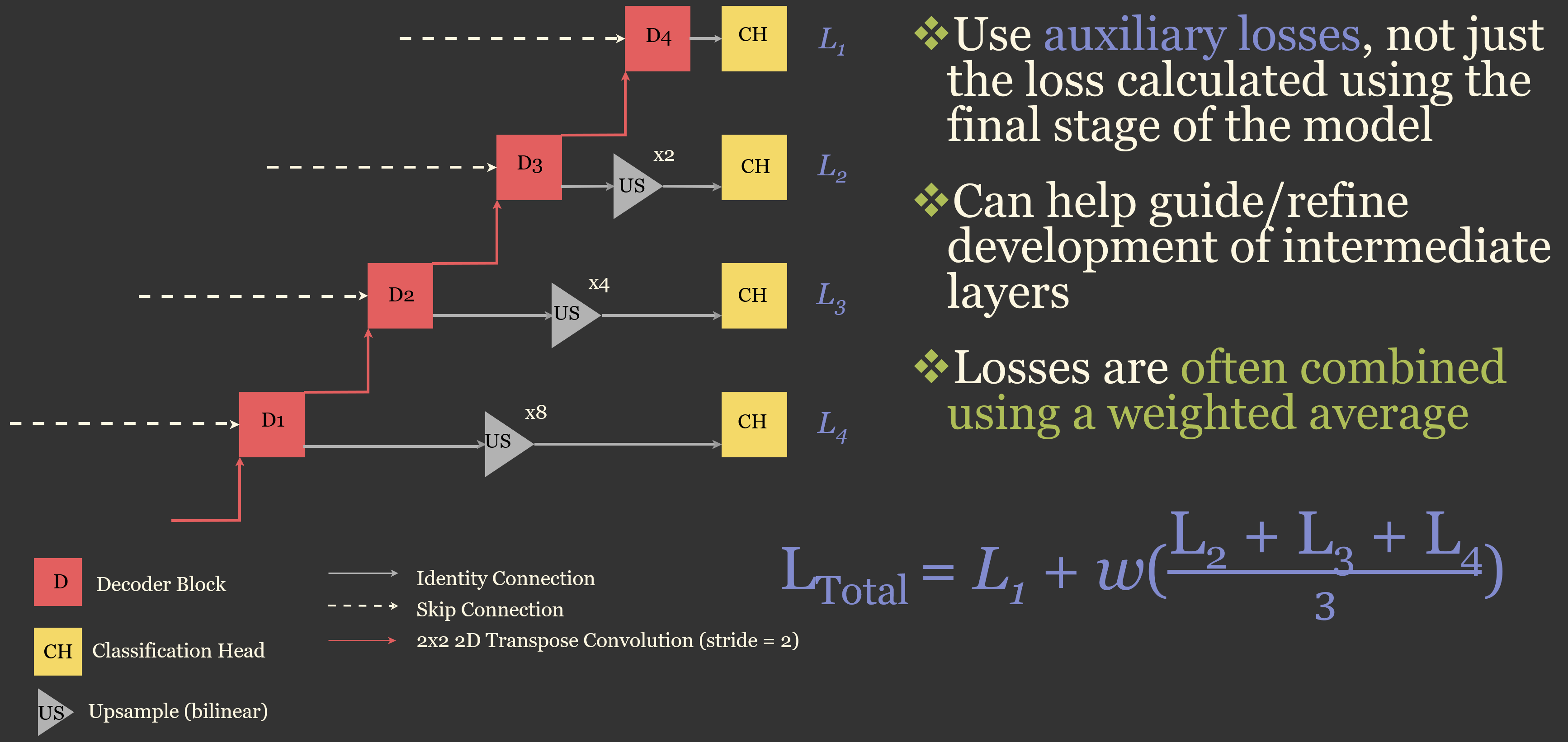
In a standard UNet, the loss is calculated only from the final output, so the earlier decoder blocks receive training signals only indirectly, through backpropagation from the final layer. With deep supervision (Lee et al., 2015), additional classification heads are attached to the earlier decoder blocks, and a loss is calculated for each of their predictions. The total loss is a weighted sum of the losses for all of the outputs. This provides more direct training signals to the intermediate layers, which can improve gradient flow and encourage the decoder to produce meaningful representations at each resolution. Deep supervision is used in several UNet variants, including UNet++ and UNet3+.
Lee, C.Y., Xie, S., Gallagher, P., Zhang, Z. and Tu, Z., 2015. “Deeply-supervised nets.” In Artificial Intelligence and Statistics (pp. 562-570). PMLR.
In our architecture, when deep supervision is enabled, a 1x1 convolution classification head is applied to the output of each of the first three decoder blocks after upsampling it to the original resolution using bilinear interpolation (by factors of 8, 4, and 2). The model then returns a list of four predictions: the final prediction followed by the predictions from the third, second, and first decoder blocks. The deep supervision heads are only used during training; for inference, only the final prediction is used. Deep supervision is conceptualized in Figure 18.9.
To train a model with deep supervision, the loss function must accept the list of predictions. The class below wraps any loss function and calculates the weighted sum of the losses for each output. The weights generally emphasize the final output.
class DeepSupervisionLoss(nn.Module):
    def __init__(self, criterion, weights=(1.0, 0.5, 0.25, 0.125)):
        super().__init__()
        self.criterion = criterion
        self.weights = weights

    def forward(self, outputs, targets):
        if not isinstance(outputs, (list, tuple)):
            return self.criterion(outputs, targets)
        return sum(w * self.criterion(o, targets) for w, o in zip(self.weights, outputs))
18.9 The Customizable UNet
We are now ready to combine these modules into a single, customizable UNet. The architecture follows the same structure as the UNet from Chapter 15: four encoder blocks separated by max pooling, a bottleneck, and four decoder blocks, each of which upsamples the features using 2D transpose convolution, concatenates the features from the associated encoder block, and applies a double convolution block. The arguments control which modules are included:
-
inChn: number of input channels -
nCls: number of classes -
actFunc: “relu”, “lrelu”, “swish”, or “gelu” -
useRes: use residual double convolution blocks in the encoder, decoder, and bottleneck (and a residual ASPP module, if used) -
useSE: apply SE modules to the output of each encoder block -
useAttn: apply attention gates along the skip connections -
useCBAM: apply CBAM modules along the skip connections (disablesuseSEanduseAttn) -
useASPP: use an ASPP module as the bottleneck -
useDS: use deep supervision -
enChn,dcChn, andbtnChn: the number of feature maps produced by each encoder block, decoder block, and the bottleneck -
dilRatesanddilChn: the dilation rates and number of feature maps for each branch of the ASPP module -
seRatio,cbamRatio, andcbamKernelSize: the reduction ratios for the SE and CBAM modules and the kernel size for the CBAM spatial attention
Figure 18.10 shows one configuration of the customizable UNet, with squeeze-and-excitation modules applied to the output of each encoder block, attention gates along the skip connections, and deep supervision. Note that this is a simplification of the architecture defined below. For example, the CBAM and ASPP modules and the residual connections are not pictured.
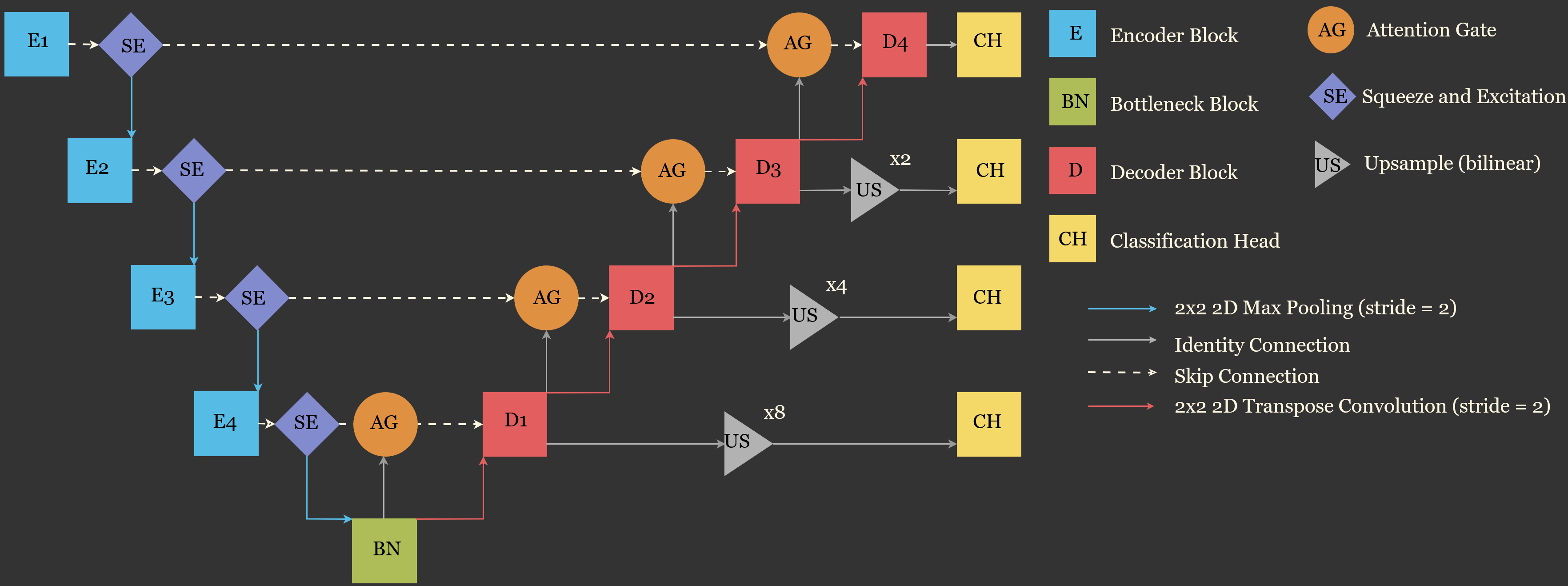
Modules that are not used are not instantiated, so they do not add parameters to the model. In the forward() method, if statements determine whether each module is applied. Note the order of operations: SE modules are applied to each encoder block’s output before max pooling; CBAM modules are applied to the encoder features along the skip connections after the bottleneck is calculated; and each attention gate is applied to the skip features immediately before they are concatenated with the decoder features, using the output of the previous decoder block (or the bottleneck) as the gating signal.
I also include a getParamGroups() method that returns optimizer parameter groups with a separate learning rate for each of the nine stages of the network (four encoder blocks, the bottleneck, and four decoder blocks), mirroring the stageLRs option in geodl. Each module is assigned to the stage in which it is applied. As discussed in Chapter 13, this allows different learning rates to be used for different components of the model, which is most useful when part of the model has been initialized with pre-trained parameters, as we will do in Chapter 27.
class defineCUNet(nn.Module):
    def __init__(self, inChn=3, nCls=2, actFunc="relu", useRes=False, useSE=False,
                 useAttn=False, useCBAM=False, useASPP=False, useDS=False,
                 enChn=(16, 32, 64, 128), dcChn=(128, 64, 32, 16), btnChn=256,
                 dilRates=(6, 12, 18), dilChn=(256, 256, 256, 256),
                 seRatio=8, cbamRatio=8, cbamKernelSize=7, negative_slope=0.01):
        super().__init__()
        if useCBAM and (useSE or useAttn):
            print("useCBAM=True: setting useSE and useAttn to False.")
            useSE, useAttn = False, False
        self.useRes, self.useSE, self.useAttn = useRes, useSE, useAttn
        self.useCBAM, self.useASPP, self.useDS = useCBAM, useASPP, useDS

        blk = DoubleConvBlkR if useRes else DoubleConvBlk
        a = dict(actFunc=actFunc, negative_slope=negative_slope)

        # Encoder
        self.e1 = blk(inChn, enChn[0], **a)
        self.e2 = blk(enChn[0], enChn[1], **a)
        self.e3 = blk(enChn[1], enChn[2], **a)
        self.e4 = blk(enChn[2], enChn[3], **a)
        if useSE:
            self.se = nn.ModuleList([SEModule(c, seRatio) for c in enChn])
        if useCBAM:
            self.cbam = nn.ModuleList([CBAMBlk(c, cbamRatio, cbamKernelSize) for c in enChn])

        # Bottleneck
        if useASPP:
            self.btn = AsppBlk(enChn[3], btnChn, dilChn=dilChn, dilRates=dilRates, useRes=useRes, **a)
        else:
            self.btn = blk(enChn[3], btnChn, **a)

        # Decoder
        upIn = [btnChn, dcChn[0], dcChn[1], dcChn[2]]
        skipChn = [enChn[3], enChn[2], enChn[1], enChn[0]]
        self.up = nn.ModuleList([
            nn.Sequential(nn.ConvTranspose2d(c, c, kernel_size=2, stride=2),
                          nn.BatchNorm2d(c), makeAct(actFunc, negative_slope))
            for c in upIn])
        self.dec = nn.ModuleList([blk(upIn[i] + skipChn[i], dcChn[i], **a) for i in range(4)])
        if useAttn:
            # Gating signal for each skip comes from the bottleneck or previous decoder block
            self.ag = nn.ModuleList([AttnBlk(skipChn[i], upIn[i]) for i in range(4)])

        # Classification heads
        self.head = nn.Conv2d(dcChn[3], nCls, kernel_size=1)
        if useDS:
            self.dsHeads = nn.ModuleList([nn.Conv2d(dcChn[i], nCls, kernel_size=1) for i in range(3)])

    def forward(self, x):
        # Encoder (SE applied before pooling)
        skips = []
        for i, enc in enumerate([self.e1, self.e2, self.e3, self.e4]):
            x = enc(x)
            if self.useSE:
                x = self.se[i](x)
            skips.append(x)
            x = F.max_pool2d(x, kernel_size=2, stride=2)

        x = self.btn(x)

        # CBAM recalibrates the skip features
        if self.useCBAM:
            skips = [self.cbam[i](s) for i, s in enumerate(skips)]

        # Decoder: deepest skip first
        skips = skips[::-1]
        decOuts = []
        for i in range(4):
            skip = self.ag[i](skips[i], x) if self.useAttn else skips[i]
            x = self.dec[i](torch.cat([self.up[i](x), skip], dim=1))
            decOuts.append(x)

        out = self.head(x)
        if self.useDS and self.training:
            # Upsample decoder blocks 3, 2, and 1 (factors of 2, 4, and 8) to full resolution
            dsOuts = [self.dsHeads[i](F.interpolate(decOuts[i], scale_factor=2**(3-i),
                                                    mode="bilinear", align_corners=False))
                      for i in (2, 1, 0)]
            return [out] + dsOuts
        return out

    def getParamGroups(self, stageLRs):
        """Return optimizer parameter groups with one learning rate per stage (9 values)."""
        assert len(stageLRs) == 9, "stageLRs must have 9 values: e1-e4, bottleneck, d1-d4"
        enc = [self.e1, self.e2, self.e3, self.e4]
        groups = []
        for i in range(4):
            mods = [enc[i]]
            if self.useSE: mods.append(self.se[i])
            if self.useCBAM: mods.append(self.cbam[i])
            groups.append(mods)
        groups.append([self.btn])
        for i in range(4):
            mods = [self.up[i], self.dec[i]]
            if self.useAttn: mods.append(self.ag[i])
            groups.append(mods)
        groups[-1].append(self.head)
        if self.useDS: groups[-1].append(self.dsHeads)
        return [{"params": [p for m in mods for p in m.parameters()], "lr": lr}
                for mods, lr in zip(groups, stageLRs)]
Note that the deep supervision outputs are only returned when the model is in training mode (self.training is True). When the model is placed in evaluation mode for validation, testing, or inference, only the final prediction is returned. This means that the validation loop and the inference code from Chapter 19 do not need to be modified.
18.10 Exploring Configurations
To check that the architecture works, I instantiate a model with all of the modules (other than CBAM) enabled and pass a random tensor through it. In training mode, a list of four predictions is returned, each with the same shape as a standard UNet prediction. In evaluation mode, a single prediction is returned.
model = defineCUNet(inChn=3, nCls=5, actFunc="swish", useRes=True, useSE=True,
                    useAttn=True, useASPP=True, useDS=True, dilRates=(2, 4, 6)).to(device)

x = torch.rand(4, 3, 256, 256).to(device)
model.train()
outs = model(x)
print([o.shape for o in outs])

model.eval()
with torch.no_grad():
    print(model(x).shape)
The modules differ in the number of parameters they add. The code below compares the total number of trainable parameters for several configurations. Note that the ASPP module adds the largest number of parameters because of its multiple 256-channel branches, while the SE modules, attention gates, and CBAM modules add relatively few.
configs = {
    "Base UNet": {},
    "Residual": {"useRes": True},
    "SE": {"useSE": True},
    "Attention gates": {"useAttn": True},
    "CBAM": {"useCBAM": True},
    "ASPP": {"useASPP": True},
    "Deep supervision": {"useDS": True},
    "Res + SE + Attn + ASPP": {"useRes": True, "useSE": True, "useAttn": True, "useASPP": True},
}
for name, kwargs in configs.items():
    m = defineCUNet(inChn=3, nCls=5, **kwargs)
    nParams = sum(p.numel() for p in m.parameters() if p.requires_grad)
print(f"{name:25s} {nParams:>12,d}")summary(defineCUNet(inChn=3, nCls=5, useAttn=True, useASPP=True), (4, 3, 256, 256), depth=3)18.11 Training with Lightning
The customizable UNet can be trained using the LitSegmenter LightningModule defined in Chapter 16. If deep supervision is not used, no changes are required. If deep supervision is used, the loss must be wrapped with the DeepSupervisionLoss class defined above, and the metrics must be calculated from only the final prediction. The subclass below handles this by overriding the _shared_step() method. During training, the model returns a list, so the first element is used for the metrics. During validation and testing, the model is in evaluation mode and returns only the final prediction.
class LitSegmenterDS(LitSegmenter):
    def _shared_step(self, batch, metrics, stage):
        x, y = batch
        outputs = self(x)
        loss = self.criterion(outputs, y)
        final = outputs[0] if isinstance(outputs, (list, tuple)) else outputs
        metrics.update(final, y)
        self.log(f"{stage}_loss", loss, on_step=False, on_epoch=True, prog_bar=True)
        self.log_dict(metrics, on_step=False, on_epoch=True, prog_bar=(stage == "val"))
        return loss
import lightning as L
from lightning.pytorch.callbacks import ModelCheckpoint
from kornia import losses
model = defineCUNet(inChn=3, nCls=5, actFunc="swish", useRes=True, useAttn=True, useDS=True)
criterion = DeepSupervisionLoss(losses.DiceLoss(average="macro"), weights=(1.0, 0.5, 0.25, 0.125))
litModel = LitSegmenterDS(model=model, nCls=5, criterion=criterion, lr=1e-4, maxLR=1e-2)
trainer = L.Trainer(max_epochs=50, accelerator="gpu", devices=1, precision="bf16-mixed",
default_root_dir="data/output/",
callbacks=[ModelCheckpoint(monitor="val_f1", mode="max")])
trainer.fit(litModel, train_dataloaders=trainDL, val_dataloaders=valDL)To use different learning rates for each stage, override configure_optimizers() and pass the result of getParamGroups() to the optimizer. In the example below, the encoder stages use a smaller learning rate than the bottleneck and decoder.
class LitSegmenterStages(LitSegmenterDS):
    def __init__(self, model, nCls, criterion, stageLRs):
        super().__init__(model, nCls, criterion)
        self.stageLRs = stageLRs

    def configure_optimizers(self):
        return torch.optim.AdamW(self.model.getParamGroups(self.stageLRs))

litModel = LitSegmenterStages(model, nCls=5, criterion=criterion,
                              stageLRs=[1e-5]*4 + [1e-4]*5)
18.12 Designing Experiments
With so many options, it is tempting to enable every module. However, adding modules does not guarantee better performance. Each module adds parameters and computations, which can increase training time and the risk of overfitting, especially with small training datasets, and the benefits of a module may depend on the characteristics of the data and the features being mapped. For example, ASPP may be most helpful when features can only be identified using broad context, while attention mechanisms may be most helpful when the features of interest occupy a small portion of each chip.
A useful approach is an ablation study, in which modules are added to or removed from a baseline model one at a time, with all other settings held constant, and the results are compared using the withheld validation or test data. Since the results of training vary between runs, as discussed in Chapter 7, each configuration should ideally be trained several times with different random seeds. The customizable UNet makes it straightforward to define these experiments, since each configuration only requires changing the arguments provided to the class.
18.13 Concluding Remarks
In this chapter, we built a variety of modules that can be added to a UNet architecture and combined them into a customizable UNet that mirrors the architecture implemented in our geodl and terrainseg packages. You can now experiment with residual connections, squeeze-and-excitation modules, attention gates, CBAM, ASPP, different activation functions, and deep supervision. Many of these modules can also be added to other architectures. In the next chapter, we will use a trained UNet to make predictions back to geospatial data over an entire image extent.
18.14 Questions
- Explain how a residual connection works. Why is a 1x1 convolution required in the shortcut path of the residual double convolution blocks used in this chapter?
- Describe the squeeze, excitation, and scale steps of a squeeze-and-excitation module. What is the purpose of the reduction ratio?
- Explain how an attention gate uses a gating signal from the decoder to filter the skip connection features. Why must the skip features be passed through a convolution with a stride of 2, and why is the attention map upsampled?
- How does the convolutional block attention module (CBAM) differ from a squeeze-and-excitation module? Why does the customizable UNet disable the SE modules and attention gates when CBAM is used?
- Explain how atrous (dilated) convolution increases the area covered by a kernel without adding parameters. What is the effective window size of a 3x3 kernel with a dilation rate of 4?
- Why might the default ASPP dilation rates of 6, 12, and 18 be inappropriate for a UNet trained using 256x256 pixel chips?
- Explain how deep supervision works and how the loss is calculated. Why are the deep supervision outputs only returned when the model is in training mode?
- What is an ablation study? Design an ablation study to assess the impact of attention gates and ASPP on a UNet trained to map a feature of your choice.