import numpy as np
import pandas as pd
import matplotlib.pyplot as plt
import math

import os

import cv2

import torch
import torch.nn as nn
from torch.nn import functional as F
from torch.utils.data.dataset import Dataset
from torch.utils.data import DataLoader

import rasterio as rio
from rasterio.plot import show

import earthpy as ep19 Spatial Predictions
19.1 Introduction
The goal of this section is to demonstrate how to use models to predict back to spatial data or full image extents as opposed to individual image chips. To accomplish this task, I create a function that accepts a trained model object and an input file and returns a raster output with the same spatial extent and coordinate reference system as the original data and one channel storing the predicted class code. At the end of this module, I will also demonstrate writing all predicted class probabilities back to disk as a multiband raster grid.
19.2 Preparation
I begin by reading in the required libraries. I will use Rasterio to read in the geospatial raster data. I will also make use of cv2 within the function for reading data. To display the resulting classification, I will use matplotlib. I also set the device to the GPU to speed up inference.
device = torch.device("cuda:0" if torch.cuda.is_available() else "cpu")
print(device)cuda:0I will use the model that was defined and trained in Chapter 16 using the Landcover.ai dataset. I first need to redefine the model architecture, instantiate an instance of the model, and move the model to the GPU. I then load the saved model parameters generated from the learning process from disk. Since the model was trained with PyTorch Lightning, the parameters are stored in the state_dict entry of the checkpoint file, and each parameter name begins with “model.” since the UNet was stored as the model attribute of the LightningModule. I remove this prefix so that the names match those of the myUNet instance. These parameters have been provided with the class data if you did not run the training process demonstrated in Chapter 16.
def double_conv(inChannels, outChannels):
  return nn.Sequential(
      nn.Conv2d(inChannels, outChannels, kernel_size=(3,3), stride=1, padding=1),
      nn.BatchNorm2d(outChannels),
      nn.ReLU(inplace=True),
      nn.Conv2d(outChannels, outChannels, kernel_size=(3,3), stride=1, padding=1),
      nn.BatchNorm2d(outChannels),
      nn.ReLU(inplace=True)
  )
def up_conv(inChannels, outChannels):
return nn.Sequential(
nn.ConvTranspose2d(inChannels, outChannels, kernel_size=(2,2), stride=2),
nn.BatchNorm2d(outChannels),
nn.ReLU(inplace=True)
)class myUNet(nn.Module):
def __init__(self, encoderChn, decoderChn, inChn, botChn, nCls):
super().__init__()
self.encoderChn = encoderChn
self.decoderChn = decoderChn
self.botChn = botChn
self.nCls = nCls
self.encoder1 = double_conv(inChn, encoderChn[0])
self.encoder2 = nn.Sequential(nn.MaxPool2d(kernel_size=2, stride=2),
double_conv(encoderChn[0], encoderChn[1]))
self.encoder3 = nn.Sequential(nn.MaxPool2d(kernel_size=2, stride=2),
double_conv(encoderChn[1], encoderChn[2]))
self.encoder4 = nn.Sequential(nn.MaxPool2d(kernel_size=2, stride=2),
double_conv(encoderChn[2], encoderChn[3]))
self.bottleneck = nn.Sequential(nn.MaxPool2d(kernel_size=2, stride=2),
double_conv(encoderChn[3], botChn))
self.decoder1up = up_conv(botChn, botChn)
self.decoder1 = double_conv(encoderChn[3]+botChn, decoderChn[0])
self.decoder2up = up_conv(decoderChn[0], decoderChn[0])
self.decoder2 = double_conv(encoderChn[2]+decoderChn[0], decoderChn[1])
self.decoder3up = up_conv(decoderChn[1], decoderChn[1])
self.decoder3 = double_conv(encoderChn[1]+decoderChn[1], decoderChn[2])
self.decoder4up = up_conv(decoderChn[2], decoderChn[2])
self.decoder4 = double_conv(encoderChn[0]+decoderChn[2], decoderChn[3])
self.classifier = nn.Conv2d(decoderChn[3], nCls, kernel_size=(1,1))
def forward(self, x):
#Encoder
encoder1 = self.encoder1(x)
encoder2 = self.encoder2(encoder1)
encoder3 = self.encoder3(encoder2)
encoder4 = self.encoder4(encoder3)
#Bottleneck
x = self.bottleneck(encoder4)
#Decoder
x = self.decoder1up(x)
x = torch.concat([x, encoder4], dim=1)
x = self.decoder1(x)
x = self.decoder2up(x)
x = torch.concat([x, encoder3], dim=1)
x = self.decoder2(x)
x = self.decoder3up(x)
x = torch.concat([x, encoder2], dim=1)
x = self.decoder3(x)
x = self.decoder4up(x)
x = torch.concat([x, encoder1], dim=1)
x = self.decoder4(x)
#Classifier head
x = self.classifier(x)
return xmodel = myUNet(encoderChn=[16,32,64,128], decoderChn=[128,64,32,16], inChn=3, botChn=512, nCls=5).to(device)saveFolder = "data/output/"
ckpt = torch.load("data/models/unetLCAI.ckpt", map_location=device)
# Lightning prefixes each parameter name with the LightningModule attribute ("model."); remove it
best_weights = {k.removeprefix("model."): v for k, v in ckpt["state_dict"].items()}
model.load_state_dict(best_weights)<All keys matched successfully>I will make a prediction to one of the provided images in the Landcover.ai dataset. I read in the image and display it using Rasterio. I selected this image because it has a mix of different land cover types within the extent. Note that the markings along the margins are the coordinates relative to the coordinate reference system to which the data are referenced.
testImg = "data/files/other/N-33-60-D-c-4-2.tif"src = rio.open(testImg)
rio.plot.show(src)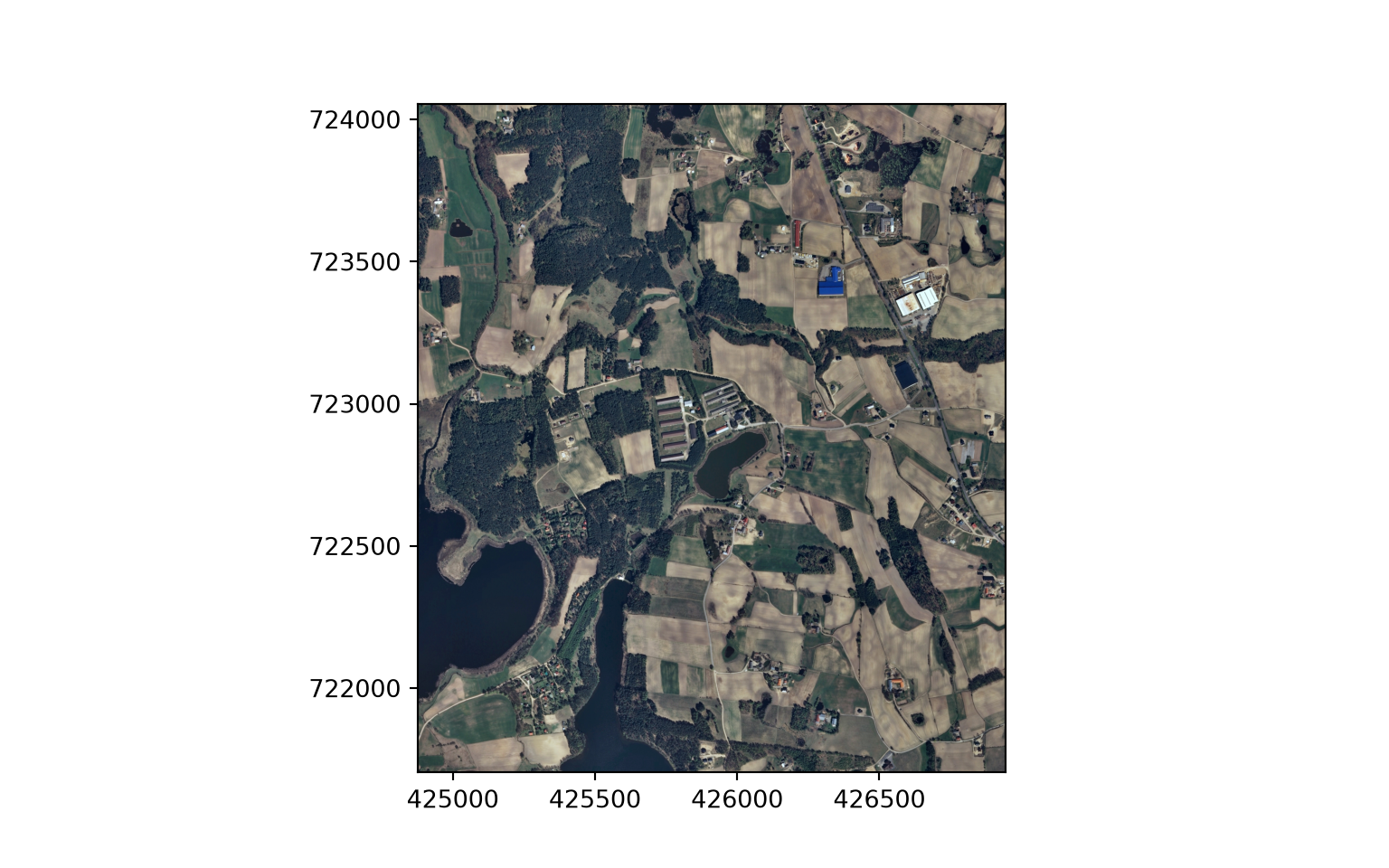
src.close()19.3 Make Classification Inference
I have defined a function below to make inferences to new data using a trained model. Here are descriptions of the input parameters.
- image_in: image to predict to. This image must have the same bands as the data used to train the model. The bands must also be in the same order as the original data. The data should be scaled using the same normalization parameters as were used in the training process.
- pred_out: name of file that will be written to disk plus the full path. Results are written as GeoTIF files with the same spatial reference information as the input image. The result will be a single band raster grid of class codes.
- model: model object that will be used to make predictions. You will need to instantiate an instance of a model and load the trained weights prior to making predictions.
- chip_size: size of image chips for processing. Although not strictly necessary, we recommend that this be the same as the chip size used to train the model.
- stride_x: stride in the x dimension (side-to-side).
- stride_y: stride in the y dimension (up-and-down).
- crop: number of columns or rows of pixels to crop from each side of the image chips while merging the output to a final product. This crop is not applied to margin chips so that the spatial extent of the output prediction is the same as the input image.
- n_channels: number of channels in the input data.
Before demonstrating this inference process, let’s discuss a few practical considerations. First, I have generally found that predictions near the edge of image chips are poorer than those in the interior. This may be due to not having a full set of neighbors when the convolution operations are applied. As a result, I recommend not using the edge pixels in the final merged output. This can be accomplished by (1) using a stride in the x and y directions that is smaller than the chip size so that each processed chip overlaps and (2) cropping the edge pixels. As noted above, as defined the function applies the defined cropping unless the chip is at the margin of the image. This is so that the spatial extent of the input image is maintained.
You may also find that very large images need to be broken into multiple smaller images, processed through the inference process separately, then merged to a final product. Images can be broken into smaller extents or tiles and the results can be merged to a final raster grid using GIS software tools, such as ArcGIS Pro or QGIS.
def geoInfer(image_in, pred_out, chip_size, stride_x, stride_y, crop, n_channels):

    #Read in topo map and convert to tensor===========================
    image1 = cv2.imread(image_in)
    image1 = cv2.cvtColor(image1, cv2.COLOR_BGR2RGB)
    image1 = image1.astype('uint8')
    image1 = torch.from_numpy(image1)
    image1 = image1.permute(2, 0, 1)
    image1 = image1.float()/255
    t_arr = image1

    #Make blank grid to write predictions two with same height and width as topo===========================
    image2 = cv2.imread(image_in)
    image2 = cv2.cvtColor(image2, cv2.COLOR_BGR2RGB)
    image2 = image2.astype('uint8')
    image2 = torch.from_numpy(image2)
    image2 = image2.permute(2, 0, 1)
    image2 = image2.float()/255
    p_arr = image2[0, :, :]
    p_arr[:,:] = 0

    #Predict to entire topo using overlapping chips, merge back to original extent=============
    size = chip_size
    stride_x = stride_x
    stride_y = stride_y
    crop = crop
    n_channels = n_channels

    across_cnt = t_arr.shape[2]
    down_cnt = t_arr.shape[1]
    tile_size_across = size
    tile_size_down = size
    overlap_across = stride_x
    overlap_down = stride_y
    across = math.ceil(across_cnt/overlap_across)
    down = math.ceil(down_cnt/overlap_down)
    across_seq = list(range(0, across, 1))
    down_seq = list(range(0, down, 1))
    across_seq2 = [(x*overlap_across) for x in across_seq]
    down_seq2 = [(x*overlap_down) for x in down_seq]
    #Loop through row/column combinations to make predictions for entire image
    for c in across_seq2:
        for r in down_seq2:
            c1 = c
            r1 = r
            c2 = c + size
            r2 = r + size
            #Default
            if c2 <= across_cnt and r2 <= down_cnt:
                r1b = r1
                r2b = r2
                c1b = c1
                c2b = c2
            #Last column
            elif c2 > across_cnt and r2 <= down_cnt:
                r1b = r1
                r2b = r2
                c1b = across_cnt - size
                c2b = across_cnt + 1
            #Last row
            elif c2 <= across_cnt and r2 > down_cnt:
                r1b = down_cnt - size
                r2b = down_cnt + 1
                c1b = c1
                c2b = c2
            #Last row, last column
            else:
                c1b = across_cnt - size
                c2b = across_cnt + 1
                r1b = down_cnt - size
                r2b = down_cnt + 1
            ten1 = t_arr[0:n_channels, r1b:r2b, c1b:c2b]
            ten1 = ten1.to(device).unsqueeze(0)
            model.eval()
            with torch.no_grad():
              ten2 = model(ten1)
            m = nn.Softmax(dim=1)
            pr_probs = m(ten2)
            ten_p = torch.argmax(pr_probs, dim=1).squeeze(1)
            ten_p = ten_p.squeeze()
            #print("executed for " + str(r1) + ", " + str(c1))
            if(r1b == 0 and c1b == 0): #Write first row, first column
                p_arr[r1b:r2b-crop, c1b:c2b-crop] = ten_p[0:size-crop, 0:size-crop]
            elif(r1b == 0 and c2b == across_cnt+1): #Write first row, last column
                p_arr[r1b:r2b-crop, c1b+crop:c2b] = ten_p[0:size-crop, 0+crop:size]
            elif(r2b == down_cnt+1 and c1b == 0): #Write last row, first column
                p_arr[r1b+crop:r2b, c1b:c2b-crop] = ten_p[crop:size+1, 0:size-crop]
            elif(r2b == down_cnt+1 and c2b == across_cnt+1): #Write last row, last column
                p_arr[r1b+crop:r2b, c1b+crop:c2b] = ten_p[crop:size, 0+crop:size+1]
            elif((r1b == 0 and c1b != 0) or (r1b == 0 and c2b != across_cnt+1)): #Write first row
                p_arr[r1b:r2b-crop, c1b+crop:c2b-crop] = ten_p[0:size-crop, 0+crop:size-crop]
            elif((r2b == down_cnt+1 and c1b != 0) or (r2b == down_cnt+1 and c2b != across_cnt+1)): # Write last row
                p_arr[r1b+crop:r2b, c1b+crop:c2b-crop] = ten_p[crop:size, 0+crop:size-crop]
            elif((c1b == 0 and r1b !=0) or (c1b ==0 and r2b != down_cnt+1)): #Write first column
                p_arr[r1b+crop:r2b-crop, c1b:c2b-crop] = ten_p[crop:size-crop, 0:size-crop]
            elif (c2b == across_cnt+1 and r1b != 0) or (c2b == across_cnt+1 and r2b != down_cnt+1): # write last column
                p_arr[r1b+crop:r2b-crop, c1b+crop:c2b] = ten_p[crop:size-crop, 0+crop:size]
            else: #Write middle chips
                p_arr[r1b+crop:r2b-crop, c1b+crop:c2b-crop] = ten_p[crop:size-crop, crop:size-crop]

    #Read in a GeoTIFF to get CRS info=======================================
    image3 = rio.open(image_in)
    profile1 = image3.profile.copy()
    image3.close()
    profile1["driver"] = "GTiff"
    profile1["dtype"] = "uint8"
    profile1["count"] = 1
    profile1["PHOTOMETRIC"] = "MINISBLACK"
    profile1["COMPRESS"] = "NONE"

    pr_out = p_arr.cpu().numpy().round().astype('uint8')

    #Write out result========================================================
    with rio.open(pred_out, "w", **profile1) as f:
        f.write(pr_out,1)

    torch.cuda.empty_cache()
I am now ready to use the function to performance inference on the image. I am using a chip size of 512-by-512 pixels since this was the size used to train the model. I am using a stride of 256 pixels in the x and y directions to allow for a 50% overlap between adjacent processing chips. I am setting the crop parameters to 50 so that the outer 50 pixels of each chip are not included in the final output unless the chip occurs on the edge of the image.
geoInfer(image_in=testImg,
    pred_out="data/output/example_pred.tif",
    chip_size=512, stride_x=256, stride_y=256, crop=50, n_channels=3)
Once the inference process executes, I read the result back in from disk and display the categorical raster using matplotlib, using a custom color map and a legend built from patches that represent each class. The link provided as a comment provides additional examples of visualizing categorical raster data. Generally, the result looks pretty good. You may want to open the file in a GIS software to explore it further and compare it to the associated image.
#https://www.earthdatascience.org/courses/use-data-open-source-python/intro-raster-data-python/raster-data-processing/classify-plot-raster-data-in-python/
from matplotlib.colors import ListedColormap, BoundaryNorm
from matplotlib.patches import Patch

clsOut = rio.open("data/output/example_pred.tif")
clsOutA = clsOut.read().squeeze()
src.close()
print(np.max(clsOutA.shape))4701classes = list(np.unique(clsOutA).astype('int'))
classColors = ['gray', 'red', 'green', 'blue', 'black']
classNames = ['background', 'building', 'woodlands', 'water', 'road']
clsBounds = BoundaryNorm([-.5, .5, 1.5, 2.5, 3.5, 4.5], len(classes))
colorMap = ListedColormap(classColors)
f, ax = plt.subplots(figsize=(10,5))
im = ax.imshow(clsOutA, cmap = colorMap, norm=clsBounds)
ax.set(title="Landcover classes")
ax.legend(handles=[Patch(facecolor=c, edgecolor="black", label=n) for c, n in zip(classColors, classNames)],
loc="center left", bbox_to_anchor=(1, 0.5))
ax.set_axis_off()
plt.show()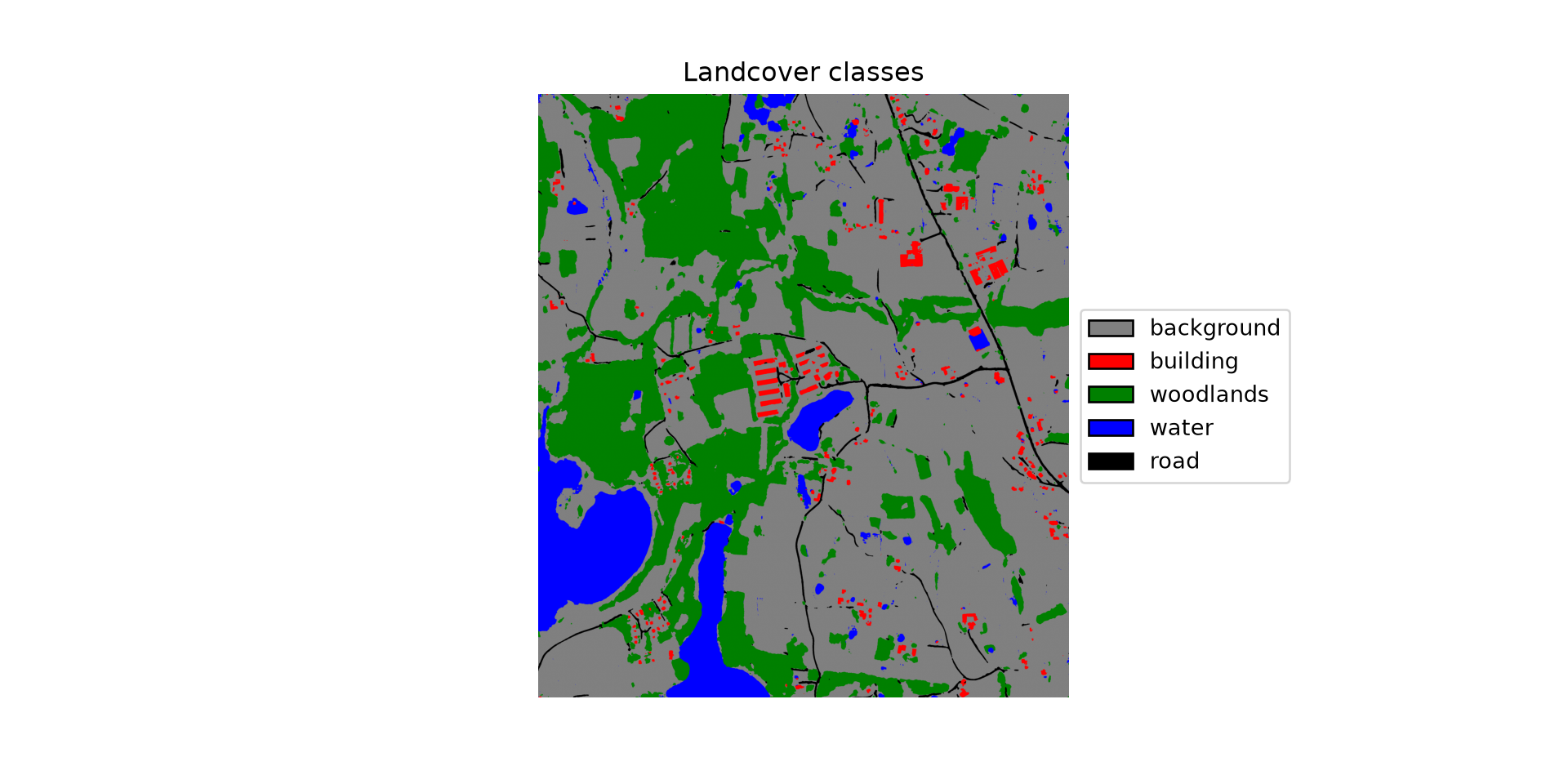
19.4 Make Probabilistic Predictions
Below I have redefined the inference function to output the predicted probability for each class as opposed to the hard classification. The result will be a multiband raster with a channel for each class. I have added a new nCls parameter which indicates the number of classes being differentiated. When predicting each chip, I do not use argmax() to obtain the index associated with the class with the highest logit. Instead, the results are passed through a softmax function to obtain class probabilities.
def geoInferProb(image_in, pred_out, nCls, chip_size, stride_x, stride_y, crop, n_channels):

    #Read in topo map and convert to tensor===========================
    image1 = cv2.imread(image_in)
    image1 = cv2.cvtColor(image1, cv2.COLOR_BGR2RGB)
    image1 = image1.astype('uint8')
    image1 = torch.from_numpy(image1)
    image1 = image1.permute(2, 0, 1)
    image1 = image1.float()/255
    t_arr = image1

    #Make blank grid to write predictions two with same height and width as topo===========================
    p_arr = torch.zeros((nCls, t_arr.shape[1], t_arr.shape[2])).float()

    #Predict to entire topo using overlapping chips, merge back to original extent=============
    size = chip_size
    stride_x = stride_x
    stride_y = stride_y
    crop = crop
    n_channels = n_channels

    across_cnt = t_arr.shape[2]
    down_cnt = t_arr.shape[1]
    tile_size_across = size
    tile_size_down = size
    overlap_across = stride_x
    overlap_down = stride_y
    across = math.ceil(across_cnt/overlap_across)
    down = math.ceil(down_cnt/overlap_down)
    across_seq = list(range(0, across, 1))
    down_seq = list(range(0, down, 1))
    across_seq2 = [(x*overlap_across) for x in across_seq]
    down_seq2 = [(x*overlap_down) for x in down_seq]
    #Loop through row/column combinations to make predictions for entire image
    for c in across_seq2:
        for r in down_seq2:
            c1 = c
            r1 = r
            c2 = c + size
            r2 = r + size
            #Default
            if c2 <= across_cnt and r2 <= down_cnt:
                r1b = r1
                r2b = r2
                c1b = c1
                c2b = c2
            #Last column
            elif c2 > across_cnt and r2 <= down_cnt:
                r1b = r1
                r2b = r2
                c1b = across_cnt - size
                c2b = across_cnt + 1
            #Last row
            elif c2 <= across_cnt and r2 > down_cnt:
                r1b = down_cnt - size
                r2b = down_cnt + 1
                c1b = c1
                c2b = c2
            #Last row, last column
            else:
                c1b = across_cnt - size
                c2b = across_cnt + 1
                r1b = down_cnt - size
                r2b = down_cnt + 1
            ten1 = t_arr[0:n_channels, r1b:r2b, c1b:c2b]
            ten1 = ten1.to(device).unsqueeze(0)
            model.eval()
            with torch.no_grad():
              ten2 = model(ten1)
            m = nn.Softmax(dim=1)
            pr_probs = m(ten2)
            ten_p = pr_probs.squeeze()
            #print("executed for " + str(r1) + ", " + str(c1))
            if(r1b == 0 and c1b == 0): #Write first row, first column
                p_arr[:, r1b:r2b-crop, c1b:c2b-crop] = ten_p[:, 0:size-crop, 0:size-crop]
            elif(r1b == 0 and c2b == across_cnt+1): #Write first row, last column
                p_arr[:,r1b:r2b-crop, c1b+crop:c2b] = ten_p[:,0:size-crop, 0+crop:size]
            elif(r2b == down_cnt+1 and c1b == 0): #Write last row, first column
                p_arr[:,r1b+crop:r2b, c1b:c2b-crop] = ten_p[:,crop:size+1, 0:size-crop]
            elif(r2b == down_cnt+1 and c2b == across_cnt+1): #Write last row, last column
                p_arr[:,r1b+crop:r2b, c1b+crop:c2b] = ten_p[:,crop:size, 0+crop:size+1]
            elif((r1b == 0 and c1b != 0) or (r1b == 0 and c2b != across_cnt+1)): #Write first row
                p_arr[:,r1b:r2b-crop, c1b+crop:c2b-crop] = ten_p[:,0:size-crop, 0+crop:size-crop]
            elif((r2b == down_cnt+1 and c1b != 0) or (r2b == down_cnt+1 and c2b != across_cnt+1)): # Write last row
                p_arr[:,r1b+crop:r2b, c1b+crop:c2b-crop] = ten_p[:,crop:size, 0+crop:size-crop]
            elif((c1b == 0 and r1b !=0) or (c1b ==0 and r2b != down_cnt+1)): #Write first column
                p_arr[:,r1b+crop:r2b-crop, c1b:c2b-crop] = ten_p[:,crop:size-crop, 0:size-crop]
            elif (c2b == across_cnt+1 and r1b != 0) or (c2b == across_cnt+1 and r2b != down_cnt+1): # write last column
                p_arr[:,r1b+crop:r2b-crop, c1b+crop:c2b] = ten_p[:,crop:size-crop, 0+crop:size]
            else: #Write middle chips
                p_arr[:,r1b+crop:r2b-crop, c1b+crop:c2b-crop] = ten_p[:,crop:size-crop, crop:size-crop]

    #Read in a GeoTIFF to get CRS info=======================================
    image3 = rio.open(image_in)
    profile1 = image3.profile.copy()
    image3.close()
    profile1["driver"] = "GTiff"
    profile1["dtype"] = "float32"
    profile1["count"] = nCls
    profile1["PHOTOMETRIC"] = "MINISBLACK"
    profile1["COMPRESS"] = "NONE"

    pr_out = p_arr.cpu().numpy().astype('float32')

    #Write out result========================================================
    with rio.open(pred_out, "w", **profile1) as f:
        f.write(pr_out)

    torch.cuda.empty_cache()
I now execute the new function for the input image. You can open each band in the resulting raster grid using your GIS software to explore the predicted class probabilities.
rpbOut = geoInferProb(image_in=testImg,
    pred_out="data/output/example_pred_prob.tif", nCls=5,
    chip_size=512, stride_x=256, stride_y=256, crop=50, n_channels=3)
Lastly, I read the result back in and display each channel, which represents the predicted probability for one class. I use the same color scale, from 0 to 1, for every class so that the maps can be compared, and the input image is included in the final panel for reference. Since the probabilities at each pixel sum to 1, areas that are bright in one map are dark in the others. Note that nearly all of the predicted probabilities are close to 0 or 1. Models trained using Dice loss tend to produce such overconfident predictions, so the probabilities should not be interpreted as well-calibrated measures of uncertainty.
probOut = rio.open("data/output/example_pred_prob.tif")
probOutA = probOut.read()
probOut.close()
print(probOutA.shape)
(5, 4701, 4136)src = rio.open(testImg)
imgA = src.read()
src.close()
f, axs = plt.subplots(2, 3, figsize=(12, 8))
axs = axs.flatten()
for i, n in enumerate(classNames):
im = axs[i].imshow(probOutA[i], cmap="viridis", vmin=0, vmax=1)
axs[i].set(title=n)
axs[i].set_axis_off()
axs[5].imshow(np.transpose(imgA, (1, 2, 0)))
axs[5].set(title="image")
axs[5].set_axis_off()
f.colorbar(im, ax=axs.tolist(), shrink=0.6, label="Predicted probability")
plt.show()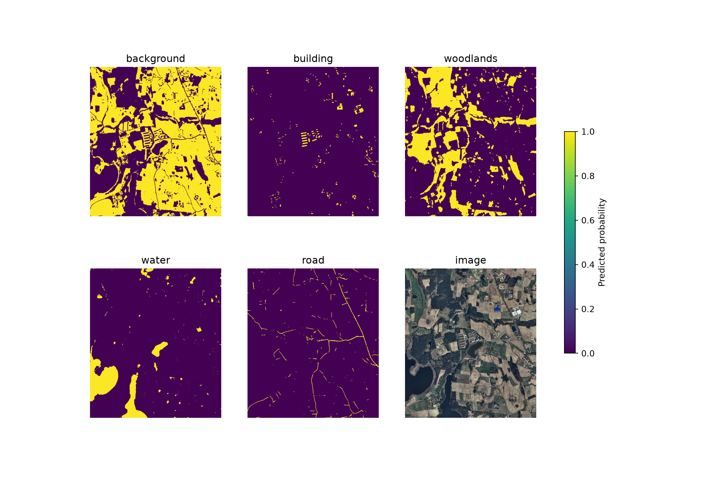
19.5 Concluding Remarks
You can now use trained models to make predictions back to geospatial data using a custom Python function that allows larger extents to be processed as overlapping image chips and subsequently reassembled to create a contiguous output. In the next chapter, we will explore the terrainseg Python package, which provides functions for generating raster masks and image chips from geospatial data and for generating chips dynamically during the training process.
19.6 Questions
- Why must the image provided for inference have the same bands, band order, and normalization as the data used to train the model?
- Why are predictions near the edges of image chips often less accurate than those in the interior of the chips?
- Explain how using overlapping chips and cropping the outer rows and columns of each chip mitigates edge effects. If a chip size of 512 pixels and a stride of 256 pixels are used, what is the overlap between adjacent chips?
- Why is the defined crop not applied to chips that occur at the margins of the image?
- Explain the difference between generating a “hard” classification and generating class probabilities. How do the two versions of the inference function differ in how the model output is processed?
- How does the inference function ensure that the output raster has the same spatial extent and coordinate reference system as the input image?
- What strategies can be used to generate predictions for very large images that cannot be processed in a single pass?
- For what applications might a multiband raster of predicted class probabilities be more useful than a single-band raster of predicted class codes?