import torch
import torch.nn as nn
import torch.nn.functional as F
from torchinfo import summary

class OverlapPatchEmbed(nn.Module):
    def __init__(self, inChn, dim, patchSize, stride):
        super().__init__()
        self.proj = nn.Conv2d(inChn, dim, kernel_size=patchSize, stride=stride, padding=patchSize // 2)
        self.norm = nn.LayerNorm(dim)

    def forward(self, x):
        x = self.proj(x)                               # (N, C, H, W)
        N, C, H, W = x.shape
        x = self.norm(x.flatten(2).transpose(1, 2))    # (N, H*W, C)
return x, H, W25 SegFormer
25.1 Introduction
All of the architectures we have explored so far rely on convolution. In this chapter, we explore transformers, an alternative architecture that relies on a mechanism called self-attention. Transformers were introduced for natural language processing (Vaswani et al., 2017) and now underlie large language models. They were adapted for computer vision with the Vision Transformer (ViT) (Dosovitskiy et al., 2021) and have since been applied to image classification, object detection, and semantic segmentation, including for remote sensing applications.
Vaswani, A., Shazeer, N., Parmar, N., Uszkoreit, J., Jones, L., Gomez, A.N., Kaiser, Ł. and Polosukhin, I., 2017. “Attention is all you need.” Advances in Neural Information Processing Systems, 30.
Dosovitskiy, A., Beyer, L., Kolesnikov, A., Weissenborn, D., Zhai, X., Unterthiner, T., Dehghani, M., Minderer, M., Heigold, G., Gelly, S. and Uszkoreit, J., 2021. “An image is worth 16x16 words: Transformers for image recognition at scale.” In International Conference on Learning Representations.
The Vision Transformer (ViT) is conceptualized in Figure 25.1. The image is divided into non-overlapping patches (e.g., 16x16 cells), and each patch is flattened and passed through a linear projection, or fully connected layer, to generate a patch embedding. A positional embedding is added to each patch embedding, and an additional learnable classification token (marked with an asterisk) is prepended to the sequence. The sequence is processed by a stack of N transformer encoder blocks, each consisting of layer normalization, multi-head self-attention, layer normalization, and an MLP, with residual connections around the attention and MLP layers. In the attention calculation, the query and key vectors are multiplied, scaled, optionally masked, and passed through a softmax to obtain the attention weights, which are multiplied by the value vectors. For classification, the output associated with the classification token is passed to an MLP head. The components of the transformer are explained in more detail in the next section.
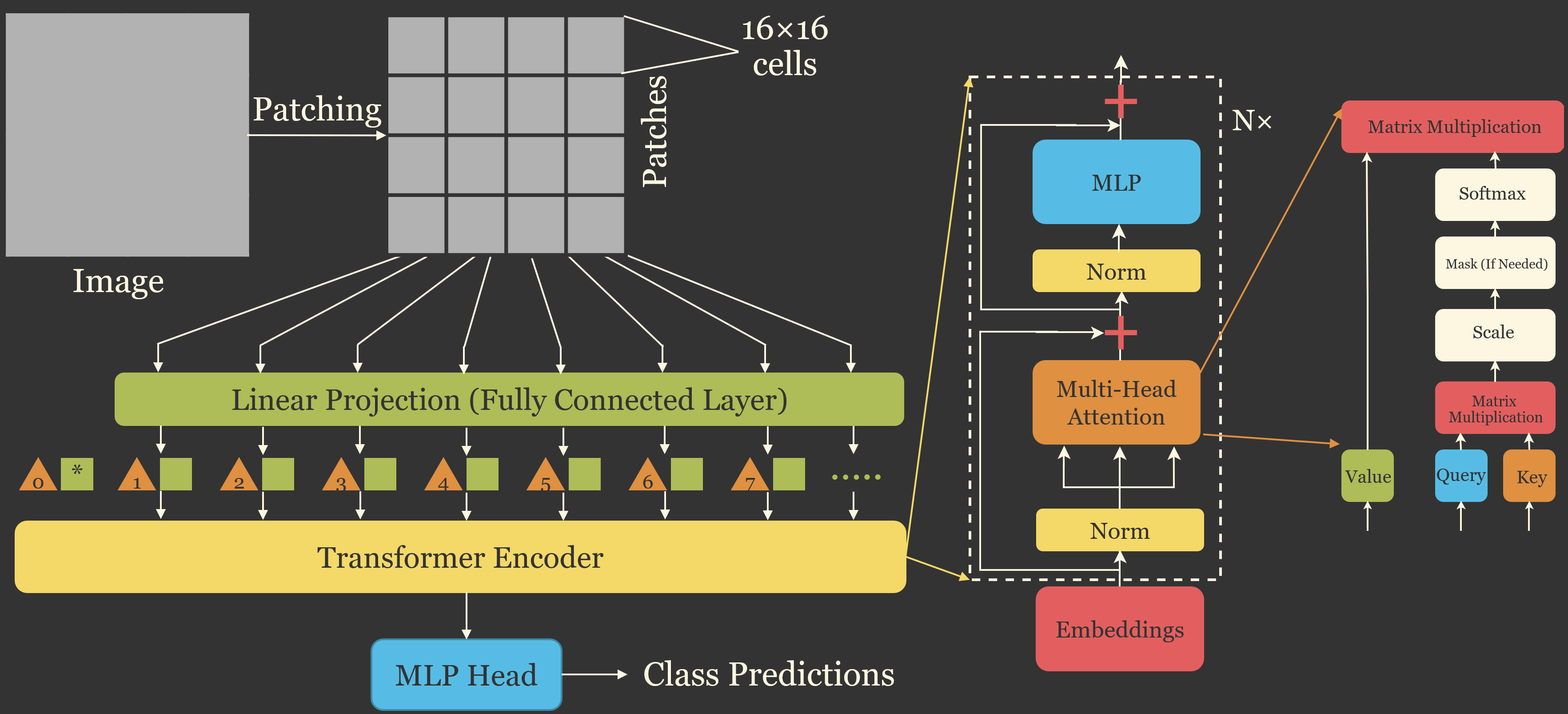
The focus of this chapter is SegFormer (Xie et al., 2021), a transformer-based architecture designed specifically for semantic segmentation. I first provide a general discussion of transformers and their strengths and weaknesses relative to CNNs. I then build the original SegFormer architecture from scratch. Finally, I use the Segmentation Models package to train a UNet that uses a pre-trained SegFormer encoder to classify the Landcover.ai dataset, as we did using a CNN-based UNet in Chapter 16. Both models are trained using PyTorch Lightning.
Xie, E., Wang, W., Yu, Z., Anandkumar, A., Alvarez, J.M. and Luo, P., 2021. “SegFormer: Simple and efficient design for semantic segmentation with transformers.” Advances in Neural Information Processing Systems, 34, pp.12077-12090.
25.2 Transformers and Self-Attention
25.2.1 Tokens and Patches
A transformer operates on a sequence of tokens, each represented by a vector of values called an embedding. In natural language processing, the tokens are words or parts of words. To apply a transformer to an image, the ViT splits the image into non-overlapping patches (e.g., 16x16 pixels), flattens each patch, and projects it to an embedding using a linear layer, which is equivalent to a convolution with a kernel size and stride equal to the patch size. A 224x224 image therefore becomes a sequence of 196 tokens. Since the operations in a transformer do not depend on the order of the tokens, a positional encoding is added to each embedding so that the model knows where each patch is located in the image.
25.2.2 Self-Attention
The core operation of a transformer is self-attention, which allows every token to gather information from every other token. For each token, three vectors are calculated using learned linear projections: a query (Q), a key (K), and a value (V). The similarity between a token’s query and every token’s key, calculated as a dot product, determines how much attention that token pays to each of the other tokens. The similarities are scaled and converted to weights that sum to 1 using a softmax function, and the output for each token is the weighted sum of all tokens’ values:
\[ \text{Attention}(Q, K, V) = \text{softmax}\left(\frac{QK^T}{\sqrt{d}}\right)V \]
where \(d\) is the length of the key vectors. In multi-head attention, this calculation is performed several times in parallel with different projections, allowing each “head” to attend to different types of relationships, and the results are concatenated.
A transformer block consists of a multi-head self-attention layer followed by a small fully connected network, often called a multilayer perceptron (MLP) or feed-forward network, which processes each token separately. Each of these is preceded by layer normalization (Chapter 24) and wrapped in a residual connection.
25.2.3 Transformers Versus CNNs
A convolutional layer only combines information within the kernel’s small window, so CNNs build up a large receptive field gradually by stacking many layers and reducing the spatial dimensions. In contrast, self-attention relates every token to every other token in a single layer, so transformers can model long-range dependencies and global context from the first layer. The weights in self-attention are also calculated from the input itself, so they adapt to each image, whereas a convolution kernel applies the same weights everywhere.
The strengths and weaknesses of transformers relative to CNNs can be summarized as follows.
Potential advantages of transformers:
- Global context: every location can use information from the entire image, which can help when features can only be identified using broad context, such as distinguishing land uses that consist of mixtures of land covers.
- Input-dependent weighting: attention weights adapt to each input.
- Scalability: transformers tend to continue improving as the size of the model and the amount of training data increase, which is why they underlie most large foundation models, including the Segment Anything Model explored in Chapter 28.
- Flexibility: the same architecture can be applied to images, text, time series, and other data types, which makes it straightforward to combine multiple data types.
Potential disadvantages of transformers:
- Weaker inductive biases: convolution assumes that nearby pixels are related (locality) and that the same pattern means the same thing anywhere in the image (translation equivariance). These assumptions are appropriate for most image data and help CNNs learn efficiently from limited data. Transformers must learn these relationships from the data, so they generally require more training data or pre-training on large datasets to outperform CNNs.
- Computational cost: the cost of self-attention grows with the square of the number of tokens. Doubling the height and width of an image increases the number of tokens by a factor of 4 and the cost of attention by a factor of 16. This is a major limitation for high-resolution imagery and for dense prediction tasks, such as semantic segmentation, which require high-resolution feature maps.
- Loss of fine detail: the ViT uses large patches and a single resolution, which is poorly suited to semantic segmentation, where detailed boundaries and multi-scale features are needed.
- Training difficulty: transformers can be more sensitive to the choice of optimizer, learning rate, warm-up, and regularization.
In practice, the distinction between the two has blurred. Hierarchical transformers, such as the Swin Transformer and the encoder of SegFormer, produce multi-scale feature maps like a CNN and use more efficient forms of attention, while modern CNNs, such as ConvNeXt (Chapter 24), have adopted many design choices from transformers. For geospatial applications with limited training data, a well-designed CNN with pre-trained weights remains a strong baseline, and the benefits of transformers are generally greatest when large pre-trained models are available.
25.3 The SegFormer Architecture
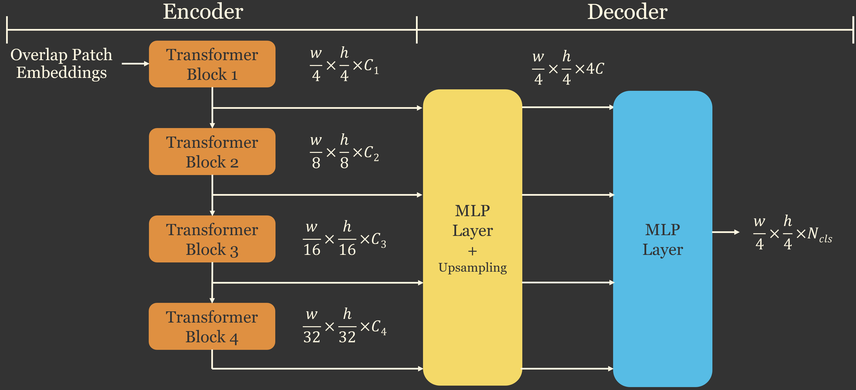
SegFormer was designed to address the limitations of the ViT for semantic segmentation. It consists of a hierarchical transformer encoder, called the Mix Transformer (MiT), and a very lightweight decoder made up entirely of fully connected (MLP) layers. The architecture is conceptualized in Figure 25.2.
25.3.1 Mix Transformer Encoder
The MiT encoder has four stages that produce feature maps at 1/4, 1/8, 1/16, and 1/32 of the input resolution, similar to the stages of a ResNet. Each stage consists of:
- Overlapping patch embedding: instead of non-overlapping patches, a convolution with a kernel larger than its stride is used to generate the tokens (a 7x7 kernel with a stride of 4 in the first stage and 3x3 kernels with a stride of 2 in the other stages). This preserves continuity between neighboring patches. The convolution also reduces the spatial dimensions, so the stages form a hierarchy.
- A sequence of transformer blocks, each consisting of efficient self-attention and a Mix-FFN.
Efficient self-attention reduces the cost of attention by spatially reducing the keys and values before the attention is calculated. With a reduction ratio of \(R\), a convolution with a kernel size and stride of \(R\) reduces the number of key and value tokens by a factor of \(R^2\), while every query token is still compared with the entire (reduced) image. The reduction ratios are 8, 4, 2, and 1 for the four stages, so the largest reduction is applied to the highest-resolution stage, where the number of tokens is largest.
The Mix-FFN inserts a 3x3 depthwise convolution between the two fully connected layers of the transformer block’s feed-forward network. The authors showed that the zero padding used in this convolution provides enough information about each token’s location that positional encodings are unnecessary. This is a practical advantage, since positional encodings learned for one image size must be interpolated when the model is applied to images of a different size, which is common in geospatial applications.
25.3.2 All-MLP Decoder
The decoder is intentionally simple. The feature maps from each of the four stages are projected to a common number of channels using a fully connected layer (equivalent to a 1x1 convolution), upsampled to 1/4 of the input resolution, concatenated, and fused using another fully connected layer. A final fully connected layer predicts the class logits at 1/4 of the input resolution, and the result is upsampled to the original resolution. Since the encoder already provides global context, a heavy decoder is not needed.
25.3.3 Model Sizes
SegFormer is available in six sizes, MiT-B0 through MiT-B5, which differ in the number of channels and transformer blocks in each stage and range from approximately 3.7 to 82 million parameters. The smallest, B0, uses 32, 64, 160, and 256 channels and 2 blocks per stage, while B2 uses 64, 128, 320, and 512 channels and 3, 4, 6, and 3 blocks.
25.4 Building SegFormer from Scratch
I now build SegFormer from scratch by subclassing nn.Module. Inside the transformer blocks, the feature maps are represented as sequences of tokens with a shape of (N, H×W, C), where each of the H×W pixel locations is a token. The flatten() and transpose() methods convert a (N, C, H, W) tensor to this shape, and the reverse operations convert it back when a convolution is needed.
The efficient self-attention layer projects the tokens to queries, keys, and values. When the reduction ratio is greater than 1, the tokens are reshaped back to a grid, reduced using a strided convolution, and normalized before the keys and values are calculated. The tensors are split into heads, and the attention is calculated using F.scaled_dot_product_attention(), which implements the equation above efficiently.
class EfficientSelfAttention(nn.Module):
    def __init__(self, dim, numHeads, srRatio):
        super().__init__()
        self.numHeads = numHeads
        self.q = nn.Linear(dim, dim)
        self.kv = nn.Linear(dim, dim * 2)
        self.proj = nn.Linear(dim, dim)
        self.srRatio = srRatio
        if srRatio > 1:
            self.sr = nn.Conv2d(dim, dim, kernel_size=srRatio, stride=srRatio)
            self.norm = nn.LayerNorm(dim)

    def forward(self, x, H, W):
        N, L, C = x.shape
        h = self.numHeads
        q = self.q(x).reshape(N, L, h, C // h).transpose(1, 2)              # (N, h, L, C/h)
        if self.srRatio > 1:
            xr = x.transpose(1, 2).reshape(N, C, H, W)
            xr = self.norm(self.sr(xr).flatten(2).transpose(1, 2))          # (N, L/R^2, C)
        else:
            xr = x
        kv = self.kv(xr).reshape(N, -1, 2, h, C // h).permute(2, 0, 3, 1, 4)
        k, v = kv[0], kv[1]                                                  # (N, h, L', C/h)
        out = F.scaled_dot_product_attention(q, k, v)                       # (N, h, L, C/h)
        return self.proj(out.transpose(1, 2).reshape(N, L, C))
The Mix-FFN expands the number of channels, applies a 3x3 depthwise convolution to the tokens reshaped as a grid, applies a GELU activation, and projects the channels back. The transformer block combines efficient self-attention and the Mix-FFN, each preceded by layer normalization and wrapped in a residual connection.
class MixFFN(nn.Module):
    def __init__(self, dim, expand=4):
        super().__init__()
        hidden = dim * expand
        self.fc1 = nn.Linear(dim, hidden)
        self.dwconv = nn.Conv2d(hidden, hidden, kernel_size=3, padding=1, groups=hidden)
        self.act = nn.GELU()
        self.fc2 = nn.Linear(hidden, dim)

    def forward(self, x, H, W):
        x = self.fc1(x)
        N, L, C = x.shape
        x = self.dwconv(x.transpose(1, 2).reshape(N, C, H, W)).flatten(2).transpose(1, 2)
        return self.fc2(self.act(x))

class TransformerBlock(nn.Module):
    def __init__(self, dim, numHeads, srRatio, expand=4):
        super().__init__()
        self.norm1 = nn.LayerNorm(dim)
        self.attn = EfficientSelfAttention(dim, numHeads, srRatio)
        self.norm2 = nn.LayerNorm(dim)
        self.ffn = MixFFN(dim, expand)

    def forward(self, x, H, W):
        x = x + self.attn(self.norm1(x), H, W)
        x = x + self.ffn(self.norm2(x), H, W)
        return x
The MiT encoder assembles four stages, each with an overlapping patch embedding, a sequence of transformer blocks, and a final layer normalization. At the end of each stage, the tokens are reshaped to a feature map, which is saved for the decoder and passed to the next stage. The default settings correspond to MiT-B0.
class MiTEncoder(nn.Module):
    def __init__(self, inChn=3, dims=(32, 64, 160, 256), depths=(2, 2, 2, 2),
                 heads=(1, 2, 5, 8), srRatios=(8, 4, 2, 1)):
        super().__init__()
        patch = [(7, 4), (3, 2), (3, 2), (3, 2)]
        inDims = (inChn,) + tuple(dims[:-1])
        self.embeds = nn.ModuleList([OverlapPatchEmbed(i, d, p, s)
                                     for i, d, (p, s) in zip(inDims, dims, patch)])
        self.stages = nn.ModuleList([
            nn.ModuleList([TransformerBlock(dims[i], heads[i], srRatios[i]) for _ in range(depths[i])])
            for i in range(4)])
        self.norms = nn.ModuleList([nn.LayerNorm(d) for d in dims])

    def forward(self, x):
        feats = []
        for embed, blocks, norm in zip(self.embeds, self.stages, self.norms):
            x, H, W = embed(x)
            for blk in blocks:
                x = blk(x, H, W)
            x = norm(x)
            x = x.transpose(1, 2).reshape(x.shape[0], -1, H, W)   # back to (N, C, H, W)
            feats.append(x)
        return feats                                              # resolutions 1/4, 1/8, 1/16, 1/32
The all-MLP decoder projects each feature map to a common number of channels using 1x1 convolutions, upsamples them to the resolution of the first stage, concatenates them, fuses them, and predicts the class logits. The full SegFormer model combines the encoder and decoder and upsamples the logits to the input resolution so that they can be compared to full-resolution masks.
class AllMLPDecoder(nn.Module):
    def __init__(self, inDims=(32, 64, 160, 256), decDim=256, nCls=2):
        super().__init__()
        self.proj = nn.ModuleList([nn.Conv2d(d, decDim, kernel_size=1) for d in inDims])
        self.fuse = nn.Sequential(nn.Conv2d(4 * decDim, decDim, kernel_size=1, bias=False),
                                  nn.BatchNorm2d(decDim), nn.ReLU(inplace=True))
        self.classifier = nn.Conv2d(decDim, nCls, kernel_size=1)

    def forward(self, feats):
        size = feats[0].shape[2:]
        x = [F.interpolate(p(f), size=size, mode="bilinear", align_corners=False)
             for p, f in zip(self.proj, feats)]
        return self.classifier(self.fuse(torch.cat(x, dim=1)))

class SegFormer(nn.Module):
    def __init__(self, inChn=3, nCls=2, dims=(32, 64, 160, 256), depths=(2, 2, 2, 2),
                 heads=(1, 2, 5, 8), srRatios=(8, 4, 2, 1), decDim=256):
        super().__init__()
        self.encoder = MiTEncoder(inChn, dims, depths, heads, srRatios)
        self.decoder = AllMLPDecoder(dims, decDim, nCls)

    def forward(self, x):
        logits = self.decoder(self.encoder(x))                     # 1/4 resolution
        return F.interpolate(logits, size=x.shape[2:], mode="bilinear", align_corners=False)
model = SegFormer(inChn=3, nCls=5) # MiT-B0 configuration
x = torch.rand(2, 3, 512, 512)
print(model(x).shape) # torch.Size([2, 5, 512, 512])
summary(model, (2, 3, 512, 512), depth=3)modelB2 = SegFormer(inChn=3, nCls=5, dims=(64, 128, 320, 512), depths=(3, 4, 6, 3),
heads=(1, 2, 5, 8), decDim=768) # MiT-B2 configuration
print(sum(p.numel() for p in modelB2.parameters()) / 1e6, "million parameters")Since the input height and width are reduced by a factor of 32 by the end of the encoder, they should be divisible by 32. Note that this from-scratch model is initialized randomly. As discussed above, transformers generally benefit greatly from pre-training, so in practice it is advisable to initialize the encoder with pre-trained weights, which we do using Segmentation Models below. Pre-trained MiT weights are also available through the Hugging Face transformers package.
The from-scratch SegFormer returns logits at the input resolution, so it can be trained using the LitSegmenter LightningModule from Chapter 16 without modification. Following the original paper, AdamW with a small learning rate and weight decay is commonly used for transformers.
import lightning as L
import segmentation_models_pytorch as smp

litSF = LitSegmenter(model=SegFormer(inChn=3, nCls=5), nCls=5,
                     criterion=smp.losses.DiceLoss(mode="multiclass", from_logits=True),
                     lr=6e-5, maxLR=6e-4)
trainer = L.Trainer(max_epochs=50, accelerator="gpu", devices=1, precision="bf16-mixed",
                    default_root_dir="data/output/")
trainer.fit(litSF, train_dataloaders=trainDL, val_dataloaders=valDL)
The data preparation used for these models is described in the next section.
25.5 UNet with a SegFormer Encoder
The Segmentation Models package provides a variety of semantic segmentation architectures along with CNN backbones that can be used as the encoder. These backbones also have pre-trained weights that can be used to implement transfer learning. Most of the available backbones are traditional CNN architectures, such as ResNet or VGGNet. However, this package also provides an implementation of the MiT encoder from SegFormer, including the B0 through B5 implementations, with parameters pre-trained on ImageNet. These encoders can be used with any of the package’s decoders, including UNet. In the remainder of this chapter, we classify the Landcover.ai dataset using a UNet architecture with a pre-trained MiT encoder. In other words, we implement UNet with an encoder based on a transformer, as opposed to CNN, architecture. As you will see, this requires very little change to the code, which is one of the great benefits of the Segmentation Models package.
25.5.1 Preparation
The preparation steps here are the same as those implemented in Chapter 16 since the same dataset is used: Landcover.ai. These DataLoaders can also be used to train the from-scratch SegFormer defined above.
- The needed libraries are imported
- The device is defined as the GPU
- The training, validation, and test sets data frames are read in
- A DataSet subclass is defined based on PyTorch’s DataSet class
- Transformations/augmentations are defined
- DataSets and DataLoaders are instantiated
Please see Chapter 16 for more details.
import numpy as np
import pandas as pd
from matplotlib import pyplot as plt
import os
import math
import cv2

import torch
import torch.nn as nn
from torch.utils.data.dataset import Dataset
from torch.utils.data import DataLoader

import albumentations as A

import segmentation_models_pytorch as smp

import torchmetrics as tm

import rasterio as rio
from rasterio.plot import show

import torchinfo
device = torch.device("cuda:0" if torch.cuda.is_available() else "cpu")
print(device)cuda:0
ImportantData Location
This chapter uses the Landcover.ai dataset, which is too large to include in the book download and must be downloaded from the source listed in Table 2. By default, the code expects the uncompressed data (the images and masks folders and the train.txt, val.txt, and test.txt files) to be saved in the data/files/landcover.ai.v1 folder and the image chips generated in Chapter 16 to be saved in the data/output/landcoverai_chips folder. If you saved the data elsewhere, set LCAI_DIR and CHIP_DIR below to the correct locations on your machine.
CLASSES = ['background', 'building', 'woodlands', 'water', 'road']
# Set these to the folder containing the train.txt, val.txt, and test.txt files and the folder containing the chips.
LCAI_DIR = "data/files/landcover.ai.v1/"
CHIP_DIR = "data/output/landcoverai_chips/"
trainDF = pd.read_csv(LCAI_DIR + "train.txt", header=None, names=["file"])
trainDF["img"] = CHIP_DIR + trainDF['file'] + ".jpg"
trainDF["mask"] = CHIP_DIR + trainDF['file'] + "_m.png"valDF = pd.read_csv(LCAI_DIR + "val.txt", header=None, names=["file"])
valDF["img"] = CHIP_DIR + valDF['file'] + ".jpg"
valDF["mask"] = CHIP_DIR + valDF['file'] + "_m.png"testDF = pd.read_csv(LCAI_DIR + "test.txt", header=None, names=["file"])
testDF["img"] = CHIP_DIR + testDF['file'] + ".jpg"
testDF["mask"] = CHIP_DIR + testDF['file'] + "_m.png"# Subclass and define custom dataset ===========================
class MultiClassSegDataset(Dataset):
def __init__(self, df, transform=None,):
self.df = df
self.transform = transform
def __getitem__(self, idx):
image_name = self.df.iloc[idx, 1]
mask_name = self.df.iloc[idx, 2]
image = cv2.imread(image_name)
image = cv2.cvtColor(image, cv2.COLOR_BGR2RGB)
mask = cv2.imread(mask_name, cv2.IMREAD_UNCHANGED)
image = image.astype('uint8')
# Masks saved as 3-band images store the same codes in each band; keep one band
if mask.ndim == 3:
mask = mask[:,:,0]
if(self.transform is not None):
transformed = self.transform(image=image, mask=mask)
image = transformed["image"]
mask = transformed["mask"]
image = torch.from_numpy(image)
mask = torch.from_numpy(mask)
image = image.permute(2, 0, 1)
image = image.float()/255
mask = mask.long()
else:
image = torch.from_numpy(image)
mask = torch.from_numpy(mask)
image = image.permute(2, 0, 1)
image = image.float()/255
mask = mask.long()
return image, mask
def __len__(self):
return len(self.df)test_transform = A.Compose(
[A.PadIfNeeded(min_height=512, min_width=512, border_mode=4), A.Resize(512, 512),]
)train_transform = A.Compose(
[
A.PadIfNeeded(min_height=512, min_width=512, border_mode=4),
A.Resize(512, 512),
A.RandomBrightnessContrast(brightness_limit=0.3, contrast_limit=0.3, p=0.5),
A.HorizontalFlip(p=0.5),
A.VerticalFlip(p=0.5),
A.MedianBlur(blur_limit=3, p=0.1),
]
)trainDS = MultiClassSegDataset(trainDF, transform=train_transform)
valDS = MultiClassSegDataset(valDF, transform=test_transform)
print("Number of Training Samples: " + str(len(trainDS)) + " Number of Testing Samples: " + str(len(valDS)))Number of Training Samples: 7470 Number of Testing Samples: 1602trainDL = DataLoader(trainDS, batch_size=8, shuffle=True, sampler=None,
batch_sampler=None, num_workers=0, collate_fn=None,
pin_memory=False, drop_last=True, timeout=0,
worker_init_fn=None)
valDL = DataLoader(valDS, batch_size=8, shuffle=False, sampler=None,
batch_sampler=None, num_workers=0, collate_fn=None,
pin_memory=False, drop_last=True, timeout=0,
worker_init_fn=None)25.5.2 Define Model
Defining a UNet model with a SegFormer backbone using Segmentation Models is very similar to defining a model using a CNN-based backbone. We simply need to provide the name of the desired SegFormer architecture as the argument for the encoder_name parameter. In the example, I am using the “mit_b2” version, which has ~24 million parameters. I am also initializing the model using parameters learned from ImageNet and not applying an activation function. The architecture is defined using the same Segmentation Models syntax that was used in the Segmentation Models module. Note that we are differentiating 5 classes, and the input data have three channels.
encoder = "mit_b2"
encoder_weights = "imagenet"
activation = None
model = smp.Unet(
encoder_name=encoder,
encoder_weights=encoder_weights,
classes=5,
activation=activation,
in_channels=3
).to(device)25.5.3 Train Model
I train the model using the LitSegmenter LightningModule from Chapter 16, which I redefine here with a constant learning rate. Training the model requires the following preparation steps:
- Define a loss metric. In this case, I use the multiclass Dice loss provided by Segmentation Models.
- Freeze the encoder. I have chosen not to train the encoder to speed up the learning process. Training the encoder may allow for improved model performance; however, this could also lead to overfitting, especially given the large number of trainable parameters in the SegFormer encoder. If you choose to train the encoder, consider using a lower learning rate for the encoder than for the decoder, as discussed in Chapter 13 and Chapter 21.
- Define the optimizer (AdamW with the default learning rate), the number of training epochs, and the location at which to save the logs and final model.
import lightning as L
from lightning.pytorch.callbacks import ModelCheckpoint
from lightning.pytorch.loggers import CSVLogger

class LitSegmenter(L.LightningModule):
    def __init__(self, model, nCls, criterion, lr=1e-3):
        super().__init__()
        self.save_hyperparameters(ignore=["model", "criterion"])
        self.model = model
        self.criterion = criterion
        self.lr = lr
        metrics = tm.MetricCollection({
            "acc": tm.Accuracy(task="multiclass", num_classes=nCls, average="micro"),
            "f1": tm.F1Score(task="multiclass", num_classes=nCls, average="macro"),
            "kappa": tm.CohenKappa(task="multiclass", num_classes=nCls),
        })
        self.train_metrics = metrics.clone(prefix="train_")
        self.val_metrics = metrics.clone(prefix="val_")
        self.test_metrics = metrics.clone(prefix="test_")

    def forward(self, x):
        return self.model(x)

    def _shared_step(self, batch, metrics, stage):
        x, y = batch
        logits = self(x)
        loss = self.criterion(logits, y)
        metrics.update(logits, y)
        self.log(f"{stage}_loss", loss, on_step=False, on_epoch=True, prog_bar=True)
        self.log_dict(metrics, on_step=False, on_epoch=True, prog_bar=(stage == "val"))
        return loss

    def training_step(self, batch, batch_idx):
        return self._shared_step(batch, self.train_metrics, "train")

    def validation_step(self, batch, batch_idx):
        self._shared_step(batch, self.val_metrics, "val")

    def test_step(self, batch, batch_idx):
        self._shared_step(batch, self.test_metrics, "test")

    def configure_optimizers(self):
        params = [p for p in self.parameters() if p.requires_grad]
        return torch.optim.AdamW(params, lr=self.lr)
#https://github.com/qubvel/segmentation_models.pytorch/issues/79
def freeze_encoder(model):
for param in model.encoder.parameters():
param.requires_grad = False
freeze_encoder(model)
criterion = smp.losses.DiceLoss(mode="multiclass", classes=5, from_logits=True, smooth=1e-8)
litModel = LitSegmenter(model=model, nCls=5, criterion=criterion, lr=1e-3)Before training the model, I print a summary of the model using torchinfo. You can see that the encoder is very different from a CNN architecture since it is made up of the components of SegFormer discussed above. Also, you can see that many of the parameters are non-trainable since I chose to freeze them.
torchinfo.summary(model, (8, 3, 512, 512))===============================================================================================
Layer (type:depth-idx) Output Shape Param #
===============================================================================================
Unet [8, 5, 512, 512] --
├─MixVisionTransformerEncoder: 1-1 [8, 3, 512, 512] --
│ └─OverlapPatchEmbed: 2-1 [8, 64, 128, 128] --
│ │ └─Conv2d: 3-1 [8, 64, 128, 128] 9,472
│ │ └─LayerNorm: 3-2 [8, 64, 128, 128] 128
│ └─Sequential: 2-2 [8, 64, 128, 128] --
│ │ └─Block: 3-3 [8, 64, 128, 128] 314,880
│ │ └─Block: 3-4 [8, 64, 128, 128] 314,880
│ │ └─Block: 3-5 [8, 64, 128, 128] 314,880
│ └─LayerNorm: 2-3 [8, 64, 128, 128] 128
│ └─OverlapPatchEmbed: 2-4 [8, 128, 64, 64] --
│ │ └─Conv2d: 3-6 [8, 128, 64, 64] 73,856
│ │ └─LayerNorm: 3-7 [8, 128, 64, 64] 256
│ └─Sequential: 2-5 [8, 128, 64, 64] --
│ │ └─Block: 3-8 [8, 128, 64, 64] 465,920
│ │ └─Block: 3-9 [8, 128, 64, 64] 465,920
│ │ └─Block: 3-10 [8, 128, 64, 64] 465,920
│ │ └─Block: 3-11 [8, 128, 64, 64] 465,920
│ └─LayerNorm: 2-6 [8, 128, 64, 64] 256
│ └─OverlapPatchEmbed: 2-7 [8, 320, 32, 32] --
│ │ └─Conv2d: 3-12 [8, 320, 32, 32] 368,960
│ │ └─LayerNorm: 3-13 [8, 320, 32, 32] 640
│ └─Sequential: 2-8 [8, 320, 32, 32] --
│ │ └─Block: 3-14 [8, 320, 32, 32] 1,656,320
│ │ └─Block: 3-15 [8, 320, 32, 32] 1,656,320
│ │ └─Block: 3-16 [8, 320, 32, 32] 1,656,320
│ │ └─Block: 3-17 [8, 320, 32, 32] 1,656,320
│ │ └─Block: 3-18 [8, 320, 32, 32] 1,656,320
│ │ └─Block: 3-19 [8, 320, 32, 32] 1,656,320
│ └─LayerNorm: 2-9 [8, 320, 32, 32] 640
│ └─OverlapPatchEmbed: 2-10 [8, 512, 16, 16] --
│ │ └─Conv2d: 3-20 [8, 512, 16, 16] 1,475,072
│ │ └─LayerNorm: 3-21 [8, 512, 16, 16] 1,024
│ └─Sequential: 2-11 [8, 512, 16, 16] --
│ │ └─Block: 3-22 [8, 512, 16, 16] 3,172,864
│ │ └─Block: 3-23 [8, 512, 16, 16] 3,172,864
│ │ └─Block: 3-24 [8, 512, 16, 16] 3,172,864
│ └─LayerNorm: 2-12 [8, 512, 16, 16] 1,024
├─UnetDecoder: 1-2 [8, 16, 512, 512] --
│ └─Identity: 2-13 [8, 512, 16, 16] --
│ └─ModuleList: 2-14 -- --
│ │ └─UnetDecoderBlock: 3-25 [8, 256, 32, 32] 2,507,776
│ │ └─UnetDecoderBlock: 3-26 [8, 128, 64, 64] 590,336
│ │ └─UnetDecoderBlock: 3-27 [8, 64, 128, 128] 147,712
│ │ └─UnetDecoderBlock: 3-28 [8, 32, 256, 256] 27,776
│ │ └─UnetDecoderBlock: 3-29 [8, 16, 512, 512] 6,976
├─SegmentationHead: 1-3 [8, 5, 512, 512] --
│ └─Conv2d: 2-15 [8, 5, 512, 512] 725
│ └─Identity: 2-16 [8, 5, 512, 512] --
│ └─Activation: 2-17 [8, 5, 512, 512] --
│ │ └─Identity: 3-30 [8, 5, 512, 512] --
===============================================================================================
Total params: 27,477,589
Trainable params: 27,477,589
Non-trainable params: 0
Total mult-adds (Units.GIGABYTES): 110.78
===============================================================================================
Input size (MB): 25.17
Forward/backward pass size (MB): 9101.64
Params size (MB): 109.91
Estimated Total Size (MB): 9236.72
===============================================================================================I am now ready to train the model. A few notes:
- I am training for a total of 25 epochs with a mini-batch size of 8 chips.
- The validation set will be predicted at the end of each training epoch in order to assess the model and monitor for overfitting.
- I am using the Dice loss and monitoring overall accuracy, class-aggregated macro-averaged F1-score, and the Kappa statistic.
- The model will only be saved if there is an improvement in the F1-score for the validation data.
If you train the model, note that it will take several hours to complete. I have provided a trained model file if you would like to run the following model assessment code without training the model.
checkpoint = ModelCheckpoint(monitor="val_f1", mode="max", save_top_k=1,
                             dirpath="data/output/sfUNetLCAI/")
trainer = L.Trainer(max_epochs=25, accelerator="gpu", devices=1, precision="bf16-mixed",
                    logger=CSVLogger("data/output/", name="sfUNetLCAI"),
                    callbacks=[checkpoint])
trainer.fit(litModel, train_dataloaders=trainDL, val_dataloaders=valDL)
25.6 Model Assessment
The remainder of the code is used to assess the trained model using the withheld testing data. This includes the following:
- Read in the training log and plot the training and validation losses and F1-scores. The log was written by Lightning’s
CSVLogger, which records the training and validation metrics for each epoch on separate rows, so I first collapse the table to one row per epoch. - Re-instantiate the model, load the saved parameters, and wrap the model in the LightningModule.
- Define the test DataSet and DataLoader.
- Calculate the aggregated metrics using the
test()method of aTrainerand the class-level metrics using a loop over the test mini-batches.
resultsDF = pd.read_csv("data/models/sfUNetLCAILogs.csv")
# Lightning writes training and validation metrics to separate rows for each epoch; collapse to one row per epoch
resultsDF = resultsDF.groupby("epoch").mean().reset_index()plt.rcParams['figure.figsize'] = [10, 10]
firstPlot = resultsDF.plot(x='epoch', y="train_loss")
resultsDF.plot(x='epoch', y="val_loss", ax=firstPlot)
plt.show()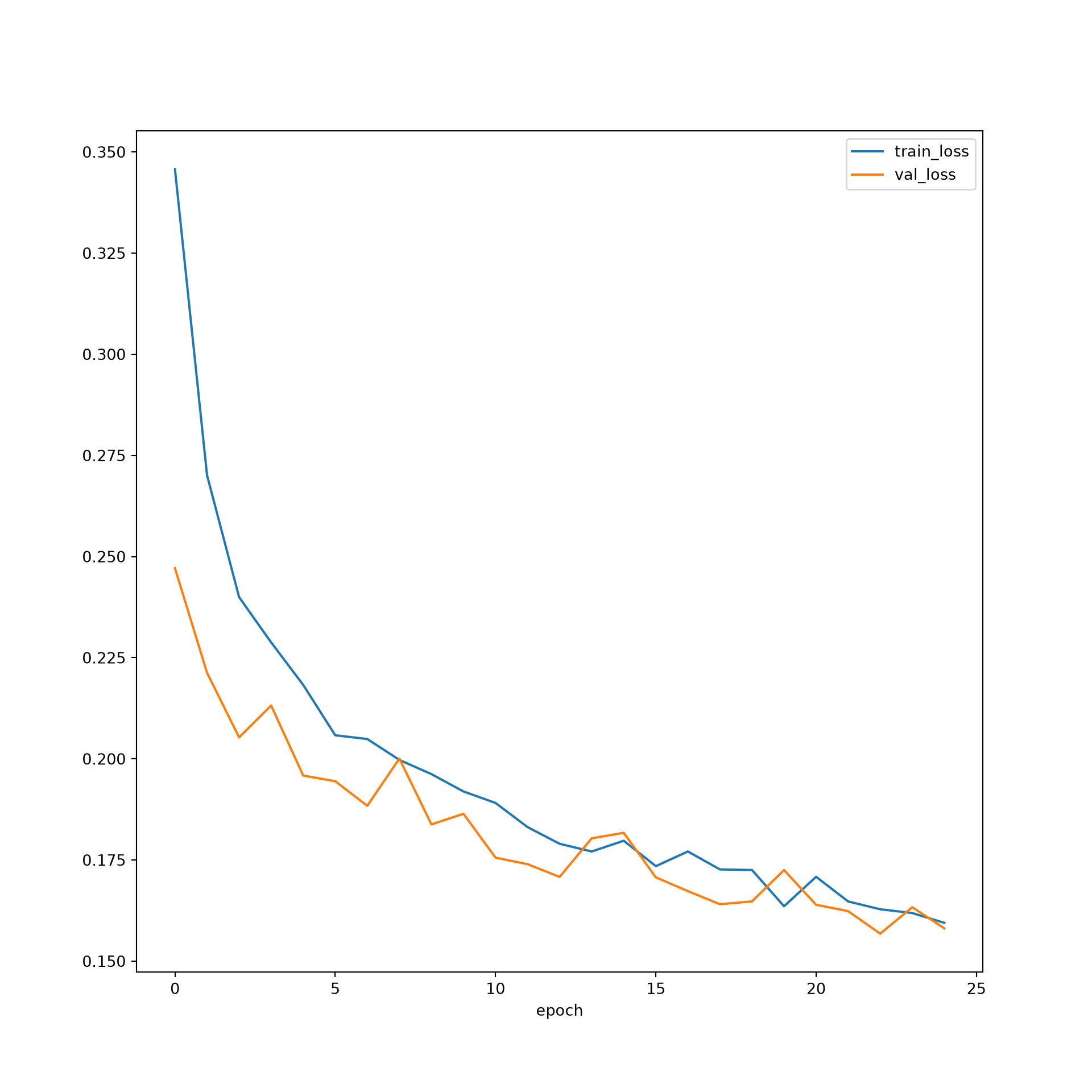
plt.rcParams['figure.figsize'] = [10, 10]
firstPlot = resultsDF.plot(x='epoch', y="train_f1")
resultsDF.plot(x='epoch', y="val_f1", ax=firstPlot)
plt.show()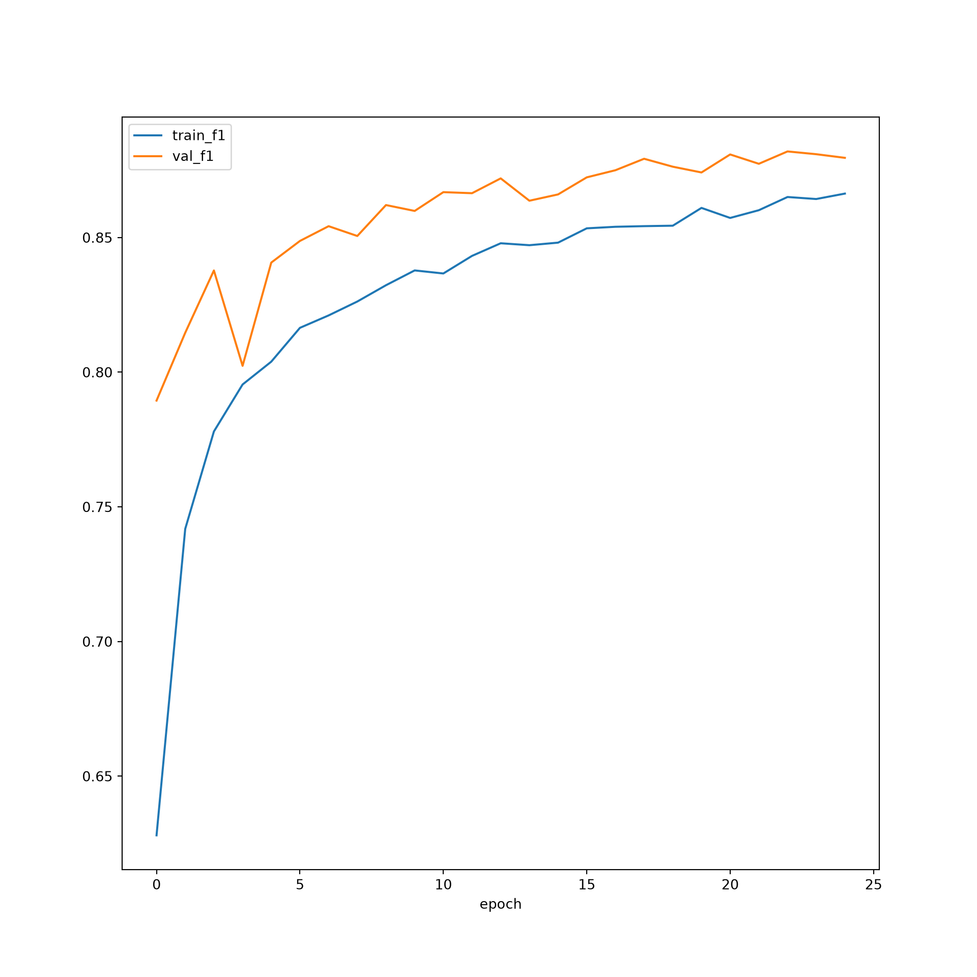
model = smp.Unet(encoder_name=encoder, encoder_weights=encoder_weights, classes=5,
                 activation=activation, in_channels=3)
criterion = smp.losses.DiceLoss(mode="multiclass", classes=5, from_logits=True, smooth=1e-8)
litModel = LitSegmenter.load_from_checkpoint("data/models/sfUNetLCAI.ckpt",
                                             model=model, criterion=criterion,
                                             map_location="cpu")

testDS = MultiClassSegDataset(testDF, transform=test_transform)
testDL = DataLoader(testDS, batch_size=8, shuffle=False, num_workers=0)

trainer = L.Trainer(accelerator="gpu", devices=1, logger=False)
trainer.test(litModel, dataloaders=testDL)
metricsCls = tm.MetricCollection({
"f1": tm.F1Score(task="multiclass", num_classes=5, average="none"),
"recall": tm.Recall(task="multiclass", num_classes=5, average="none"),
"precision": tm.Precision(task="multiclass", num_classes=5, average="none"),
"cm": tm.ConfusionMatrix(task="multiclass", num_classes=5),
}).to(device)
litModel = litModel.to(device).eval()
with torch.no_grad():
for inputs, targets in testDL:
inputs, targets = inputs.to(device), targets.to(device)
metricsCls.update(litModel(inputs), targets)
for k, v in metricsCls.compute().items():
print(k, v)25.7 Concluding Remarks
In this chapter, we explored transformers and the self-attention mechanism, compared their strengths and weaknesses to those of CNNs, built the original SegFormer architecture from scratch, and trained a UNet with a pre-trained SegFormer encoder using Segmentation Models and PyTorch Lightning. Using Segmentation Models, a transformer-based encoder could be used with very minimal changes to the code. Since transformer-based architectures can capture spatial context over broad spatial extents, you may want to experiment with SegFormer as opposed to CNN-based architectures. However, training an architecture that includes transformer components may require more training data, or pre-trained weights, in order to see improvement relative to a CNN-based architecture.
25.8 Questions
- Explain how an image is converted to a sequence of tokens for input to a Vision Transformer. Why are positional encodings needed, and why does SegFormer not use them?
- Explain how self-attention is calculated using queries, keys, and values. What is the purpose of multi-head attention?
- Compare transformers and CNNs in regard to their receptive fields and inductive biases. Why do transformers generally require more training data or pre-training than CNNs?
- Why does the computational cost of self-attention limit its use for high-resolution imagery? How does SegFormer’s efficient self-attention reduce this cost?
- Explain how overlapping patch embedding differs from the patch embedding used in the Vision Transformer, and how it produces a hierarchy of feature maps.
- Describe the Mix-FFN and the all-MLP decoder used in SegFormer. Why can SegFormer use such a lightweight decoder?
- Why was the SegFormer encoder frozen when training the UNet in this chapter? What are the potential trade-offs of training the encoder, and how could different learning rates be used if it is trained?
- Design an experiment to compare a UNet with a SegFormer encoder to a UNet with a ResNet-34 encoder for the Landcover.ai dataset. What settings should be held constant, and what metrics would you use to compare the models?