8 Statistical Inference
8.1 Topics Covered
- Distinguish a population from a sample, and a parameter from a statistic
- Explain what a sampling distribution is and why it is the foundation of inference
- Build and interpret confidence intervals using both theory (the t distribution) and simulation (the bootstrap)
- Carry out hypothesis tests using two complementary approaches: theory-based (distribution) tests and simulation-based (permutation) tests
- Choose, execute, and interpret a t-test, ANOVA, and chi-square test, along with their nonparametric alternatives
- Perform pairwise comparisons and explain why multiple testing requires an adjustment
- Reason about statistical power, effect size, and the difference between statistical and practical significance
- Recognize how spatial autocorrelation violates the independence assumption behind most of these tests, and what to do about it
8.2 Why Inference?
In earlier chapters you learned to import, clean, summarize, and visualize data. Those skills describe data. Statistical inference is about using the data you have to say something with about data you don’t have with an associated estimate of uncertainty. Every inferential question in this chapter has the same shape:
I observed some pattern in a sample. How confident can I be that the pattern also exists in the population the sample came from, or could it plausibly be the product of random chance?
8.3 Packages and Data
In this chapter, we use the tidyverse packages for general data wrangling and summarization, the infer and broom packages for statistical inference, and spdep for assessing spatial autocorrelation. We also make heavy use of statistical test made available by base R. For our example data, we use the pdxTrees package, which provides inventories of trees collected by Portland Parks & Recreation’s Urban Forestry volunteers. We specifically use the parks inventory, which records tens of thousands of trees across Portland’s public parks, including size, condition, species, origin, and location. We first simplify and clean the dataset to better suite our needs.
parks_raw <- get_pdxTrees_parks()

trees <- parks_raw |>
  rename_with(tolower) |>
  transmute(
    park,
    latitude, longitude,
    genus, common_name,
    dbh,                                   # diameter at breast height (in)
    tree_height,                           # ft
    carbon_storage_lb,
    native = if_else(native == "Yes", "Native", "Non-native"),
    condition = factor(condition, levels = c("Good", "Fair", "Poor", "Dead")),
    functional_type = recode(functional_type,
      BD = "Broadleaf deciduous", BE = "Broadleaf evergreen",
      CD = "Conifer deciduous",   CE = "Conifer evergreen"
    ),
    mature_size = factor(mature_size, levels = c("S", "M", "L"))
  ) |>
  drop_na(dbh, tree_height, native, condition, functional_type) |>
  filter(dbh > 0, tree_height > 0)

glimpse(trees)
Rows: 25,118
Columns: 12
$ park <chr> "Gammans Park", "Gammans Park", "Gammans Park", "Gam…
$ latitude <dbl> 45.57491, 45.57489, 45.57493, 45.57490, 45.57491, 45…
$ longitude <dbl> -122.6936, -122.6938, -122.6942, -122.6939, -122.694…
$ genus <chr> "Pseudotsuga", "Pseudotsuga", "Crataegus", "Quercus"…
$ common_name <chr> "Douglas-Fir", "Douglas-Fir", "Lavalle Hawthorn", "N…
$ dbh <dbl> 37.4, 32.5, 9.7, 10.3, 33.2, 32.1, 28.4, 27.2, 35.2,…
$ tree_height <dbl> 105, 94, 23, 28, 102, 95, 103, 105, 97, 112, 112, 48…
$ carbon_storage_lb <dbl> 3223.3, 2460.8, 310.3, 400.1, 2533.4, 2333.7, 1874.5…
$ native <chr> "Native", "Native", "Non-native", "Non-native", "Nat…
$ condition <fct> Fair, Fair, Fair, Poor, Fair, Fair, Fair, Fair, Fair…
$ functional_type <chr> "Conifer evergreen", "Conifer evergreen", "Broadleaf…
$ mature_size <fct> L, L, S, L, L, L, L, L, L, L, L, L, L, M, S, S, S, S…Before running any test, it is good practice to look at the categories you plan to compare. Category labels (e.g., "Yes"/"No" for native) occasionally change between package versions, so confirm these counts look sensible.
trees |> count(native)# A tibble: 2 × 2
native n
<chr> <int>
1 Native 10922
2 Non-native 14196trees |> count(condition)# A tibble: 3 × 2
condition n
<fct> <int>
1 Good 1641
2 Fair 22150
3 Poor 1327trees |> count(functional_type)# A tibble: 4 × 2
functional_type n
<chr> <int>
1 Broadleaf deciduous 13975
2 Broadleaf evergreen 242
3 Conifer deciduous 192
4 Conifer evergreen 107098.4 A Field Guide to Common Statistical Tests
Before diving into details, Table 8.1 gives a map of the tests used in this chapter (and a few related tests). Use it as a reference: the right test depends on the question you are asking and the type of variables involved.
| Test | Typical question | Variables | Key assumptions | Base R | Nonparametric / simulation alternative | How to interpret a small p-value |
|---|---|---|---|---|---|---|
| One-sample t-test | Is the mean equal to some reference value? | 1 numeric | Independent obs.; roughly normal or large n | t.test(x, mu = ) |
Wilcoxon signed-rank (wilcox.test(x, mu = )); bootstrap CI |
The population mean likely differs from the reference value |
| Two-sample t-test (Welch) | Do two groups have different means? | Numeric ~ 2-level categorical | Independent obs. within & between groups; roughly normal or large n | t.test(y ~ g) |
Wilcoxon rank-sum / Mann–Whitney (wilcox.test(y ~ g)); permutation test |
The two population means likely differ |
| Paired t-test | Did values change within the same units? | 2 numeric measures on the same units | Differences are independent and roughly normal | t.test(x, y, paired = TRUE) |
Wilcoxon signed-rank on differences; permutation of signs | The mean within-unit difference is likely not zero |
| One-way ANOVA | Do 3+ groups have different means? | Numeric ~ categorical (3+ levels) | Independence; normal residuals; equal variances (or use Welch’s ANOVA) |
aov(), oneway.test()
|
Kruskal–Wallis (kruskal.test()); permutation F test |
At least one group mean differs — follow up with pairwise comparisons |
| Pairwise comparisons | Which groups differ? | Numeric ~ categorical | Same as ANOVA; adjust for multiple tests |
TukeyHSD(), pairwise.t.test()
|
pairwise.wilcox.test() |
The specific pair differs, after controlling for the number of comparisons |
| Chi-square test of independence | Are two categorical variables associated? | Categorical × categorical | Independent obs.; expected counts ≥ 5 in (nearly) all cells | chisq.test(table) |
Fisher’s exact test (fisher.test()); permutation chi-square |
The distribution of one variable differs across levels of the other |
| Chi-square goodness of fit | Do observed category frequencies match expected ones? | 1 categorical | Independent obs.; expected counts ≥ 5 | chisq.test(x, p = ) |
Simulated p-value (simulate.p.value = TRUE) |
Observed frequencies depart from the hypothesized proportions |
| Test of proportions | Do two groups have different proportions? | Binary ~ categorical | Independence; enough successes/failures | prop.test() |
Permutation or bootstrap of the difference in proportions | The population proportions likely differ |
| Correlation | Are two numeric variables linearly (or monotonically) related? | Numeric × numeric | Independence; linearity (Pearson) | cor.test() |
Spearman / Kendall (method = "spearman"); permutation |
A nonzero association likely exists in the population |
| Moran’s I | Are nearby observations more similar than distant ones? | Numeric + locations | A sensible definition of “neighbor” | spdep::moran.test() |
spdep::moran.mc() (permutation) |
Values are spatially clustered — observations are not independent |
A p-value is not:
- the probability that the null hypothesis is true,
- the probability that your result was “due to chance,”
- a measure of how large or important an effect is.
A p-value is the probability of observing a statistic at least as extreme as yours, if the null hypothesis were true.
8.5 Populations, Samples, and Sampling Distributions
8.5.1 Parameters and Statistics
- A population is the entire set of units you want to learn about (e.g., all trees in all public parks in Portland).
- A parameter is a numeric summary of the population (e.g., the true mean diameter at breast height (DBH) for all trees in public parks in Portland, \(\mu\)).
- A sample is the subset of units you actually observe (e.g., a subset of trees occurring in public parks in Portland).
- A statistic is a numeric summary of the sample (e.g., the sample mean, \(\bar{x}\)), used to estimate the parameter (the mean DBH of a subset of trees occurring in public parks in Portland).
In real research we almost never see the whole population. For teaching purposes in this chapter, we will pretend the park inventory is the entire population of Portland park trees. That lets us do something impossible in practice: compare our sample estimates to the true answer.
population <- trees

pop_mean_dbh <- mean(population$dbh)
pop_mean_dbh
[1] 20.767678.5.2 Demo: One Sample is Not the Truth
Let’s draw a single random sample of 30 trees multiple times. By selecting out a random sample of 30 trees from the entire population multiple times, you can see that we do not obtain the same mean each time. This sampling variability is the central problem inference solves.
sample_30 <- population |> slice_sample(n = 30)
mean(sample_30$dbh)
[1] 22.01333sample_30 <- population |> slice_sample(n = 30)
mean(sample_30$dbh)[1] 21.7sample_30 <- population |> slice_sample(n = 30)
mean(sample_30$dbh)[1] 24.41667sample_30 <- population |> slice_sample(n = 30)
mean(sample_30$dbh)[1] 20.03sample_30 <- population |> slice_sample(n = 30)
mean(sample_30$dbh)[1] 16.736678.5.3 Demo: The Sampling Distribution
If we drew many samples and computed the mean of each, the distribution of those means is called the sampling distribution. The infer function rep_slice_sample() makes this easy.
sample_means <- map_dfr(c(10, 30, 100), \(n) {
  population |>
    rep_slice_sample(n = n, reps = 1000) |>
    summarize(xbar = mean(dbh)) |>
    mutate(n = n)
})

ggplot(sample_means, aes(xbar)) +
  geom_histogram(bins = 40, fill = "forestgreen", color = "white") +
  geom_vline(xintercept = pop_mean_dbh, linewidth = 1, linetype = "dashed") +
  facet_wrap(~ n, ncol = 1, labeller = label_both) +
  labs(x = "Sample mean DBH (in)", y = "Count",
       title = "Sampling distributions of the mean DBH",
       subtitle = "Dashed line = population mean")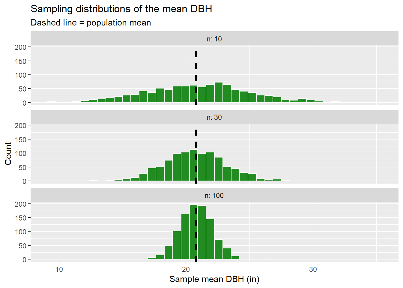
Notice three things:
- Centered on the truth: sample means are centered on the population mean: the sample mean is an unbiased estimator.
- Gets narrower as n grows: the spread of the sampling distribution, the standard error, shrinks in proportion to \(1/\sqrt{n}\).
- Becomes bell-shaped: even though DBH itself is strongly right-skewed (check with a histogram), the distribution of sample means becomes approximately normal. This is the Central Limit Theorem, and it is why t-tests work reasonably well on non-normal data when samples are large.
# A tibble: 3 × 3
      n simulated_se theoretical_se
  <dbl>        <dbl>          <dbl>
1    10         4.17           4.24
2    30         2.40           2.45
3   100         1.29           1.34
Every inference procedure needs an approximation of the sampling distribution. There are two ways to get one:
-
Theory (distribution-based): mathematics tells us the sampling distribution follows a known shape (normal, t, F, \(\chi^2\)) under certain assumptions. This is what
t.test(),aov(), andchisq.test()do. - Simulation (resampling-based): we use the computer to build the sampling distribution by resampling the data (bootstrapping for confidence intervals, permuting for hypothesis tests). This is what the infer package does.
When assumptions hold, the two approaches agree closely. When they disagree, that is a signal to look harder at your data.
8.6 Confidence Intervals
A confidence interval (CI) gives a range of plausible values for a parameter. Its width communicates our uncertainty.
8.6.1 Theory-Based CI with Base R
t.test(sample_30$dbh)$conf.int[1] 12.19639 21.27694
attr(,"conf.level")
[1] 0.958.6.2 Bootstrap CI with infer
The bootstrap idea: treat the sample as a stand-in for the population, and resample from the sample, with replacement, to see how much the statistic varies.
The infer workflow uses a consistent set of verbs:
| Verb | Purpose |
|---|---|
| specify() | Which variable(s) are we studying? |
| hypothesize() | What is the null hypothesis? (tests only) |
| generate() | Simulate new data (bootstrap or permute) |
| calculate() | Compute the statistic for each simulated data set |
| visualize() | Plot the simulated distribution |
| get_confidence_interval() / get_p_value() | Summarize |
boot_dist <- sample_30 |>
  specify(response = dbh) |>
  generate(reps = 2000, type = "bootstrap") |>
  calculate(stat = "mean")

boot_ci <- boot_dist |>
  get_confidence_interval(level = 0.95, type = "percentile")
boot_ci
# A tibble: 1 × 2
lower_ci upper_ci
<dbl> <dbl>
1 12.8 21.0visualize(boot_dist) +
shade_confidence_interval(endpoints = boot_ci) +
labs(x = "Bootstrap mean DBH (in)")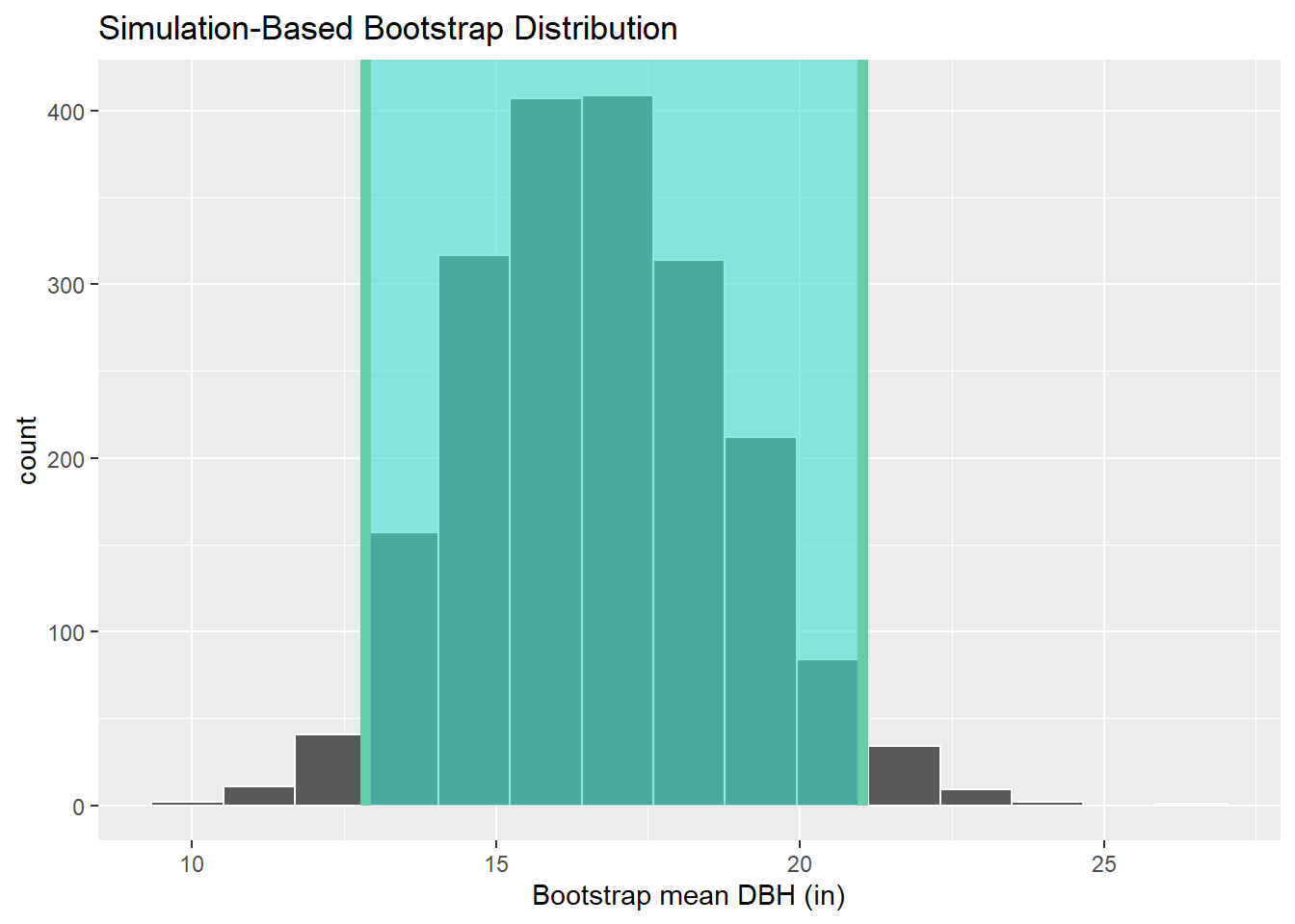
8.6.3 Demo: What “95% Confidence” Actually Means
“95% confident” does not mean there is a 95% probability the true mean is inside this particular interval. It means that the method produces intervals that capture the true parameter about 95% of the time across repeated samples. Because we have the “population,” we can check this directly.
[1] 0.97ggplot(ci_sim, aes(y = replicate, xmin = conf.low, xmax = conf.high,
color = captures)) +
geom_linerange() +
geom_vline(xintercept = pop_mean_dbh, linetype = "dashed") +
scale_color_manual(values = c(`TRUE` = "grey50", `FALSE` = "firebrick")) +
labs(x = "95% CI for mean DBH (in)", y = "Sample",
color = "Captures true mean?",
title = "100 confidence intervals from 100 random samples")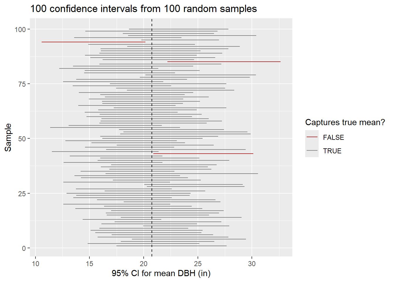
Change n = 30 to n = 100. What happens to the widths of the intervals? What happens to the capture rate? Then change the confidence level with t.test(dbh, conf.level = 0.80).
8.7 The Logic of Hypothesis Testing
Every hypothesis test follows the same recipe:
- State a null hypothesis (\(H_0\), “nothing interesting is going on”) and an alternative hypothesis (\(H_A\)).
- Choose a test statistic that measures the departure from \(H_0\).
- Find the null distribution: how the statistic would vary if \(H_0\) were true.
- Compare the observed statistic to the null distribution to get a p-value.
- Make a decision at a pre-chosen significance level \(\alpha\) (commonly 0.05) and, more importantly, interpret in context.
| \(H_0\) is true | \(H_0\) is false | |
|---|---|---|
| Reject \(H_0\) | Type I error (rate = \(\alpha\)) | Correct (rate = power) |
| Fail to reject | Correct | Type II error (rate = \(\beta\)) |
The permutation test makes step 3 intuitive: if group labels truly don’t matter (\(H_0\)), then shuffling them shouldn’t change anything. So we shuffle the labels many times, recompute the statistic each time, and see where our real statistic falls.
8.8 Comparing Two Groups: The t-test
Question: Do native and non-native park trees differ in mean trunk diameter (diameter at breast height or DBH)?
8.8.1 Explore First
We can use summary statistics and grouped box plots to compare the central tendency and distribution of DBH for native and non-native trees for the entire population. The results suggest that the native trees have a larger DBH on average.
# A tibble: 2 × 5
  native         n mean_dbh median_dbh sd_dbh
  <chr>      <int>    <dbl>      <dbl>  <dbl>
1 Native     10922     24.9       25.8   12.8
2 Non-native 14196 17.6 14.8 12.9ggplot(trees, aes(native, dbh)) +
geom_boxplot(fill = "darkseagreen", outlier.alpha = 0.2) +
scale_y_log10() +
labs(x = NULL, y = "DBH (in, log scale)")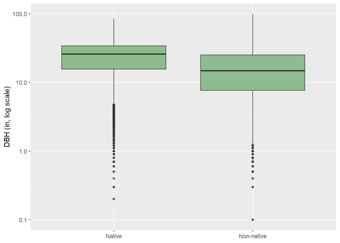
8.8.2 Working with a Sample
Testing on the full inventory of tens of thousands of trees would make nearly any difference “significant”. To mimic a realistic field study, we’ll take a random sample of 60 trees per group.
tree_sample <- trees |>
  group_by(native) |>
  slice_sample(n = 60) |>
  ungroup()
8.8.3 Theory-Based: Welch’s t-test in Base R
t_res <- t.test(dbh ~ native, data = tree_sample)
t_res
    Welch Two Sample t-test

data:  dbh by native
t = 1.9404, df = 114.05, p-value = 0.05479
alternative hypothesis: true difference in means between group Native and group Non-native is not equal to 0
95 percent confidence interval:
 -0.09662045  9.34662045
sample estimates:
    mean in group Native mean in group Non-native
                23.99333                 19.36833
R uses Welch’s t-test by default, which does not assume equal variances. This is almost always the better choice; use var.equal = TRUE only with good reason. The test suggests that the two groups do have different mean DBHs since the obtained p-value (0.011) is lower than the pre-defined threshold (0.05).
8.8.4 Simulation-Based: Permutation Test with infer
We now use the infer package to implement a permutation test. This test also suggests statistical difference since the obtained p-value (0.006) is lower than our predefined threshold (0.05). We are testing for differences in means between the two groups. The null hypothesis is that the the mean DBH is not different between the two groups (or, mean DBH is independent of group). The data are permuted 2,000 times to estimate the population distribution, and we then compare the difference in means between the two groups to this distribution.
obs_diff <- tree_sample |>
  specify(dbh ~ native) |>
  calculate(stat = "diff in means", order = c("Native", "Non-native"))

null_diff <- tree_sample |>
  specify(dbh ~ native) |>
  hypothesize(null = "independence") |>
  generate(reps = 2000, type = "permute") |>
  calculate(stat = "diff in means", order = c("Native", "Non-native"))

visualize(null_diff) +
  shade_p_value(obs_stat = obs_diff, direction = "two-sided")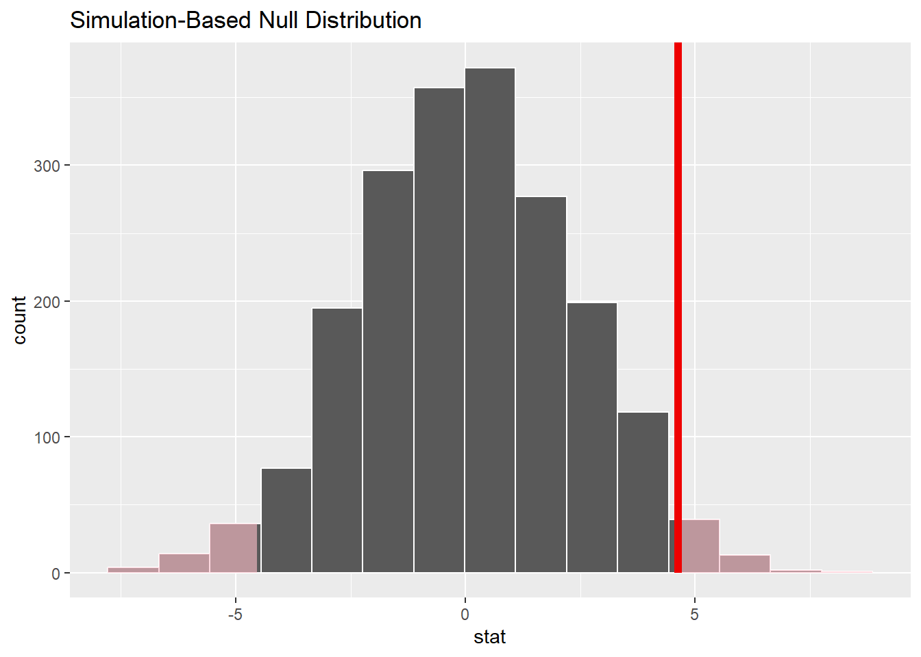
get_p_value(null_diff, obs_stat = obs_diff, direction = "two-sided")# A tibble: 1 × 1
p_value
<dbl>
1 0.049We next obtain confidence intervals for the estimate generated using permutation. Note that the range does not include zero. The range is also pretty similar to the results we obtained when using the t-test implemented with base R.
boot_diff <- tree_sample |>
  specify(dbh ~ native) |>
  generate(reps = 2000, type = "bootstrap") |>
  calculate(stat = "diff in means", order = c("Native", "Non-native"))

get_confidence_interval(boot_diff, level = 0.95, type = "percentile")
# A tibble: 1 × 2
lower_ci upper_ci
<dbl> <dbl>
1 0.0737 8.93infer also wraps theory-based tests in tidy syntax, e.g. t_test(tree_sample, dbh ~ native, order = c("Native", "Non-native")), and lets you overlay the theoretical t distribution on a simulated null with visualize(method = "both").
8.8.5 Effect Size
A p-value tells you whether a difference is detectable; an effect size tells you whether it is meaningful. Cohen’s d expresses the mean difference in standard deviation units (rough guide: 0.2 small, 0.5 medium, 0.8 large). Our results suggest a medium to larger effect size. In short, the difference in mean DBH between the two groups is likely meaningful.
# A tibble: 1 × 3
   diff pooled_sd cohens_d
  <dbl>     <dbl>    <dbl>
1  4.62      13.1    0.354
8.8.6 Checking Assumptions and a Nonparametric Alternative
DBH is right-skewed. With 60 per group the Central Limit Theorem gives us some protection, but it’s worth checking. The historgrams and QQ-plots generated below suggest non-normality or a right-skewed distribution, especially for the non-native trees.
ggplot(tree_sample, aes(x = dbh)) +
  geom_density()+
  facet_wrap(~ native)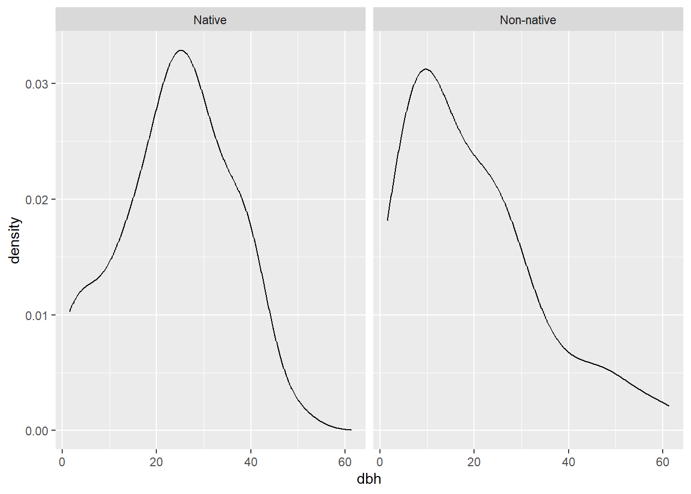
ggplot(tree_sample, aes(sample = dbh)) +
  stat_qq() + stat_qq_line() +
  facet_wrap(~ native)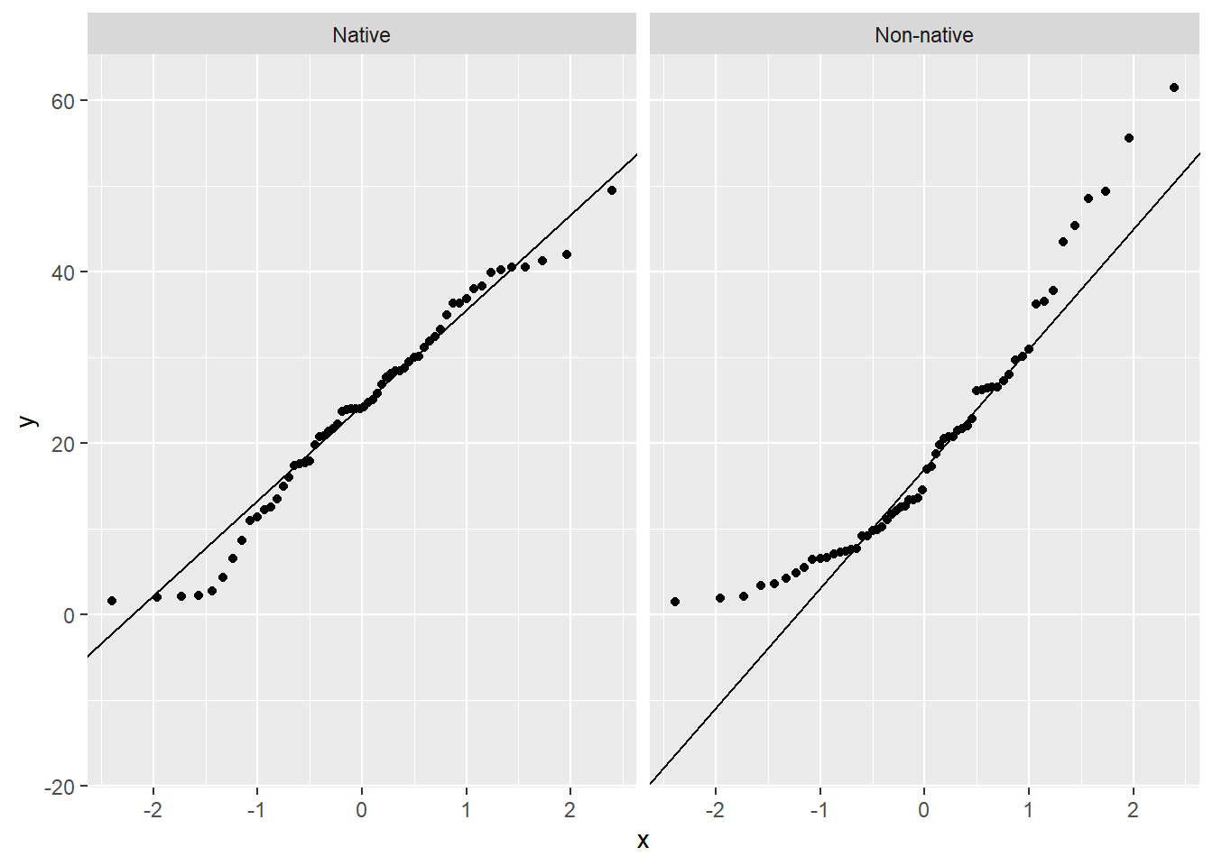
When data are skewed or contain outliers, the Wilcoxon rank-sum test (also called Mann–Whitney U) compares groups using ranks rather than raw values. It asks whether values in one group tend to be larger than in the other group. As with the parametric tests above, this test suggests statistical significance since the obtained p-value (0.005) is lower than our pre-defined threshold (0.05).
wilcox.test(dbh ~ native, data = tree_sample, conf.int = TRUE)
    Wilcoxon rank sum test with continuity correction

data:  dbh by native
W = 2275, p-value = 0.01275
alternative hypothesis: true location shift is not equal to 0
95 percent confidence interval:
  1.400055 11.300015
sample estimates:
difference in location
               6.59994
Nonparametric tests trade a little power (when parametric assumptions hold) for robustness (when they don’t). Note also that they often test a slightly different hypothesis (e.g., Wilcoxon is about the location shift / stochastic ordering, not the mean).
8.9 Comparing Three or More Groups: ANOVA
Question: Does mean tree height differ among functional types (broadleaf/conifer, deciduous/evergreen)?
Why not just run a t-test on every pair? Because each test carries a chance of a false positive, and those chances add up. ANOVA asks one omnibus question first: is there any difference among the group means at all? Looking at the grouped box plots below, it would appear that at least some of the groups are different. For example, conifer evergreen tends to be taller than the other groups. As a result, this is worth exploring statistically.
# A tibble: 4 × 4
  functional_type         n mean_height sd_height
  <chr>               <int>       <dbl>     <dbl>
1 Broadleaf deciduous    40        46.2      25.7
2 Broadleaf evergreen    40        29.2      18.5
3 Conifer deciduous      40        51.4      30.6
4 Conifer evergreen 40 87.4 41.4ggplot(height_sample, aes(functional_type, tree_height)) +
geom_boxplot(fill = "darkseagreen") +
labs(x = NULL, y = "Tree height (ft)")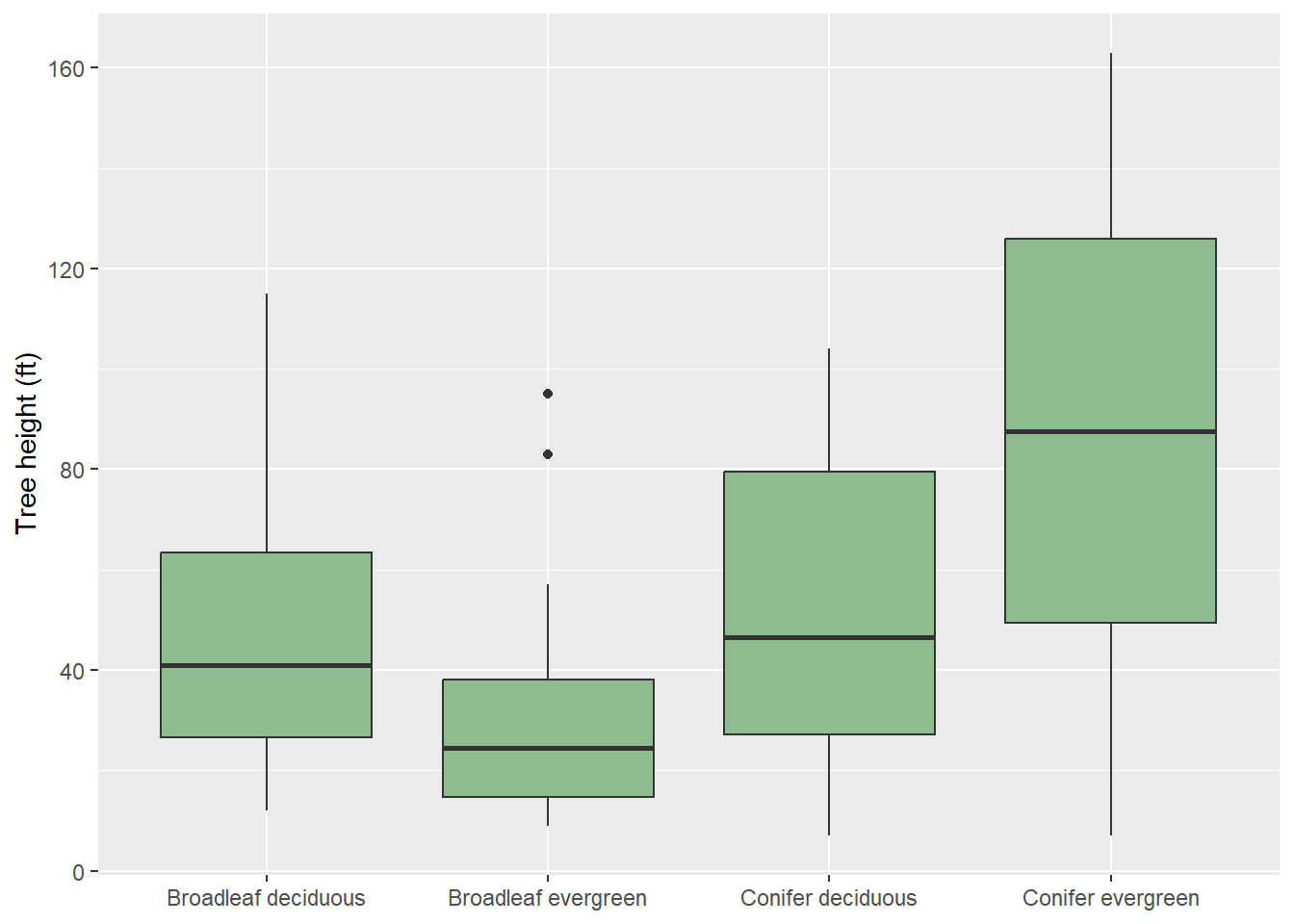
If a functional type has fewer than 40 trees in the inventory, slice_sample() will simply return all of them.
8.9.1 Theory-Based: aov() and Welch’s ANOVA
The F statistic compares variation between group means to variation within groups. Large F = group means are farther apart than within-group noise would suggest. The results of this test generally suggest statistical significance (very low p-value). Note that this test does not offer any information about which pairs of groups are different.
                 Df Sum Sq Mean Sq F value   Pr(>F)
functional_type   3  72040   24013   26.32 7.86e-14 ***
Residuals       156 142326     912
---
Signif. codes:  0 '***' 0.001 '**' 0.01 '*' 0.05 '.' 0.1 ' ' 1
# Welch's ANOVA does not assume equal variances
oneway.test(tree_height ~ functional_type, data = height_sample)
    One-way analysis of means (not assuming equal variances)

data:  tree_height and functional_type
F = 23.614, num df = 3.000, denom df = 83.624, p-value = 3.635e-11
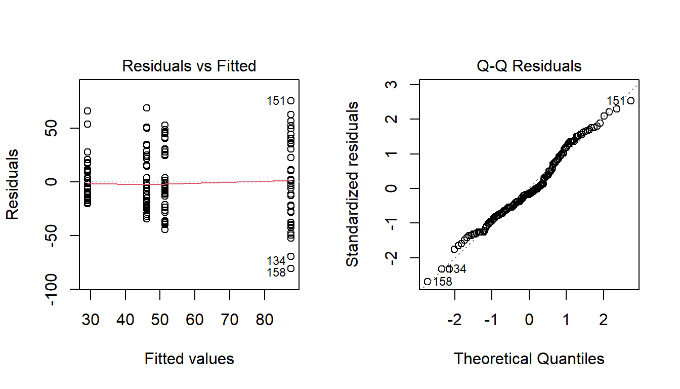
Since the ANOVA tests has assumptions, it is necessary to explore any issues that may invalidate the results. This includes homoscedasticity (the residual or error does not vary with the values of the variable being predicted) and normality of the residuals. Plotting the fitted values against the residuals should show no trend, and a QQ-plot should show limited divergence from the 1:1 line. Generally, the graphs below suggest these assumptions are not violated.
8.9.2 Simulation-Based: Permutation F Test with infer
We now execute the test using a permutation-based method via the infer package. The results also suggest statistical difference based on the obtained p-value.
obs_F <- height_sample |>
  specify(tree_height ~ functional_type) |>
  calculate(stat = "F")

null_F <- height_sample |>
  specify(tree_height ~ functional_type) |>
  hypothesize(null = "independence") |>
  generate(reps = 2000, type = "permute") |>
  calculate(stat = "F")

visualize(null_F, method = "both") +
  shade_p_value(obs_stat = obs_F, direction = "greater")
Warning: Check to make sure the conditions have been met for the theoretical method.
infer currently does not check these for you.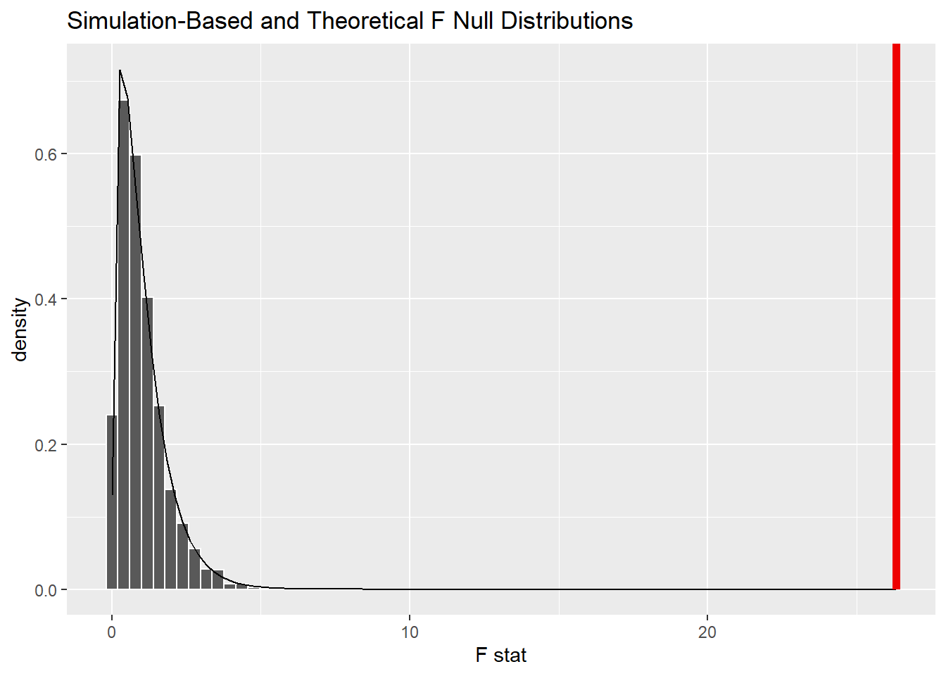
get_p_value(null_F, obs_stat = obs_F, direction = "greater")Warning: Please be cautious in reporting a p-value of 0. This result is an approximation
based on the number of `reps` chosen in the `generate()` step.
ℹ See `get_p_value()` (`?infer::get_p_value()`) for more information.# A tibble: 1 × 1
p_value
<dbl>
1 0The method = "both" option overlays the theoretical F distribution on the permutation distribution — a nice visual check of whether the two engines agree.
8.9.3 Nonparametric Alternative: Kruskal–Wallis
Here, we demonstrate the Kruskal-Wallis test, a nonparametric alternative to ANOVA that is based on ranks. The null hypothesis of this test is that all groups come from the same distribution or that the population distributions are identical. Similar two the two ANOVA implementations demonstrated above, this test suggests statistical difference between at least two of the groups.
kruskal.test(tree_height ~ functional_type, data = height_sample)
    Kruskal-Wallis rank sum test

data:  tree_height by functional_type
Kruskal-Wallis chi-squared = 47.482, df = 3, p-value = 2.744e-10
8.9.4 Pairwise Comparisons
A significant ANOVA tells you some means differ, but not which pair(s) of means differ. Pairwise comparisons answer that follow-up question.
Tukey’s Honest Significant Differences gives adjusted p-values and simultaneous confidence intervals for every pair. Intervals that do not cross zero indicate pairs that differ. In this example, three of the six pairs are suggested to be different. Specifically, the conifer evergreen group is suggested to be different from the other three groups while the other three groups are suggested to not be different from each other. This confirms what we saw visually in the grouped box plot above.
tukey <- TukeyHSD(anova_fit)
tukey
Tukey multiple comparisons of means
95% family-wise confidence level
Fit: aov(formula = tree_height ~ functional_type, data = height_sample)
$functional_type
diff lwr upr p adj
Broadleaf evergreen-Broadleaf deciduous -17.00 -34.539864 0.5398644 0.0611847
Conifer deciduous-Broadleaf deciduous 5.15 -12.389864 22.6898644 0.8711582
Conifer evergreen-Broadleaf deciduous 41.25 23.710136 58.7898644 0.0000000
Conifer deciduous-Broadleaf evergreen 22.15 4.610136 39.6898644 0.0069580
Conifer evergreen-Broadleaf evergreen 58.25 40.710136 75.7898644 0.0000000
Conifer evergreen-Conifer deciduous 36.10 18.560136 53.6398644 0.0000019tidy(tukey) |>
ggplot(aes(estimate, contrast, xmin = conf.low, xmax = conf.high)) +
geom_pointrange() +
geom_vline(xintercept = 0, linetype = "dashed") +
labs(x = "Difference in mean height (ft), 95% family-wise CI", y = NULL)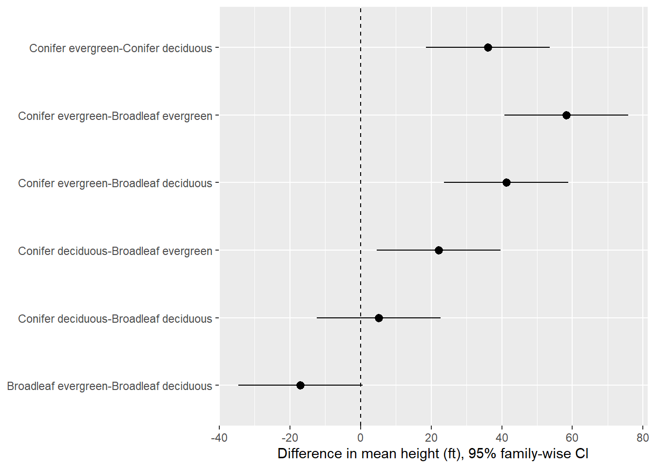
There are other options available including the pairwise t-test with Holm adjustment and the nonparametric pairwise Wilcox test, which is often performed after a statistically significant result from the Kruskal-Wallis test.
# Pairwise t-tests with Holm adjustment (no equal-variance assumption)
pairwise.t.test(height_sample$tree_height, height_sample$functional_type,
                p.adjust.method = "holm", pool.sd = FALSE)
    Pairwise comparisons using t tests with non-pooled SD

data:  height_sample$tree_height and height_sample$functional_type

                    Broadleaf deciduous Broadleaf evergreen Conifer deciduous
Broadleaf evergreen 0.00223             -                   -
Conifer deciduous   0.41712             0.00066             -
Conifer evergreen   5.9e-06             3.7e-10             0.00013

P value adjustment method: holm
# Nonparametric pairwise comparisons following Kruskal–Wallis
pairwise.wilcox.test(height_sample$tree_height, height_sample$functional_type,
p.adjust.method = "holm")
    Pairwise comparisons using Wilcoxon rank sum exact test

data:  height_sample$tree_height and height_sample$functional_type

                    Broadleaf deciduous Broadleaf evergreen Conifer deciduous
Broadleaf evergreen 0.00172             -                   -
Conifer deciduous   0.46798             0.00161             -
Conifer evergreen   1.5e-05             1.3e-10             0.00034

P value adjustment method: holm
8.9.5 Demo: Why We Adjust for Multiple Comparisons
If each test has a 5% false-positive rate, the chance of at least one false positive across \(m\) independent tests is \(1 - 0.95^m\).
tibble(m = 1:20, familywise_error = 1 - 0.95^m) |>
  ggplot(aes(m, familywise_error)) +
  geom_line() + geom_point() +
  geom_hline(yintercept = 0.05, linetype = "dashed") +
  labs(x = "Number of tests", y = "P(at least one false positive)")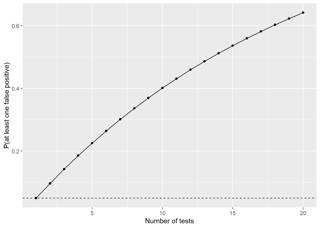
Let’s verify by simulation. We’ll create six fake groups by randomly assigning labels (so we know for certain that \(H_0\) is true) and count how often any of the 15 pairwise comparisons comes out “significant.” Without adjustment, we’d “discover” a difference between random groups far more than 5% of the time.
any_sig <- function(adjust) {
  d <- population |>
    slice_sample(n = 120) |>
    mutate(fake_group = sample(rep(LETTERS[1:6], each = 20)))
  p <- pairwise.t.test(d$dbh, d$fake_group, p.adjust.method = adjust)$p.value
  any(p < 0.05, na.rm = TRUE)
}

tibble(
  adjustment = c("none", "holm"),
  familywise_error = map_dbl(adjustment, \(a) mean(replicate(500, any_sig(a))))
)
# A tibble: 2 × 2
adjustment familywise_error
<chr> <dbl>
1 none 0.348
2 holm 0.0428.10 Associations Between Categorical Variables: Chi-Square
Question: Is tree condition associated with whether a tree is native?
In contrast to the methods discussed above, the chi-square test allows you to explore the association between two categorical variables. In our example, we specifically explore whether the proportions of tree conditions vary between native and non-native trees.
cond_sample <- trees |>
  slice_sample(n = 600) |>
  mutate(condition = droplevels(condition))   # drop any category absent from the sample

cond_tab <- table(cond_sample$native, cond_sample$condition)
cond_tab
             Good Fair Poor
  Native       16  245   13
Non-native 20 295 11prop.table(cond_tab, margin = 1) |> round(3)
              Good  Fair  Poor
  Native     0.058 0.894 0.047
Non-native 0.061 0.905 0.034ggplot(cond_sample, aes(native, fill = condition)) +
geom_bar(position = "fill") +
scale_fill_brewer(palette = "RdYlGn", direction = -1) +
labs(x = NULL, y = "Proportion", fill = "Condition")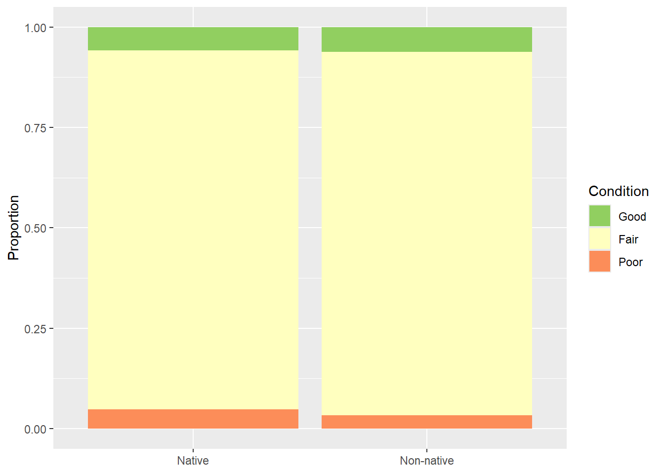
The chi-square statistic compares observed counts to the counts we’d expect if the two variables were independent. Below, we perform this analysis using the theory-based approach, as implemented with base R, followed by the permutation-based approach using infer. Both methods generally suggest that the difference in proportions or counts in condition classes do not vary between native and non-native trees (i.e., the p-values are above the 0.05 threshold). This seems to support the visualization provided in the graph above, were proportions are not drastically different between the two groups.
chi_res <- chisq.test(cond_tab)
chi_res
    Pearson's Chi-squared test

data:  cond_tab
X-squared = 0.73963, df = 2, p-value = 0.6909
# Always check expected counts (rule of thumb: >= 5)
chi_res$expected |> round(1)
             Good  Fair Poor
  Native     16.4 246.6   11
  Non-native 19.6 293.4   13
# Standardized residuals show which cells drive the result (|r| > 2 is notable)
chi_res$stdres |> round(2)
              Good  Fair  Poor
  Native     -0.15 -0.44  0.85
  Non-native  0.15  0.44 -0.85
“Dead” trees are rare, so some expected counts may be below 5. When that happens, the \(\chi^2\) approximation is unreliable. Options: combine sparse categories (e.g., “Poor” + “Dead”), use chisq.test(..., simulate.p.value = TRUE), use fisher.test(), or use a permutation test.
obs_chisq <- cond_sample |>
  specify(condition ~ native) |>
  calculate(stat = "Chisq")

null_chisq <- cond_sample |>
  specify(condition ~ native) |>
  hypothesize(null = "independence") |>
  generate(reps = 2000, type = "permute") |>
  calculate(stat = "Chisq")

visualize(null_chisq, method = "both") +
  shade_p_value(obs_stat = obs_chisq, direction = "greater")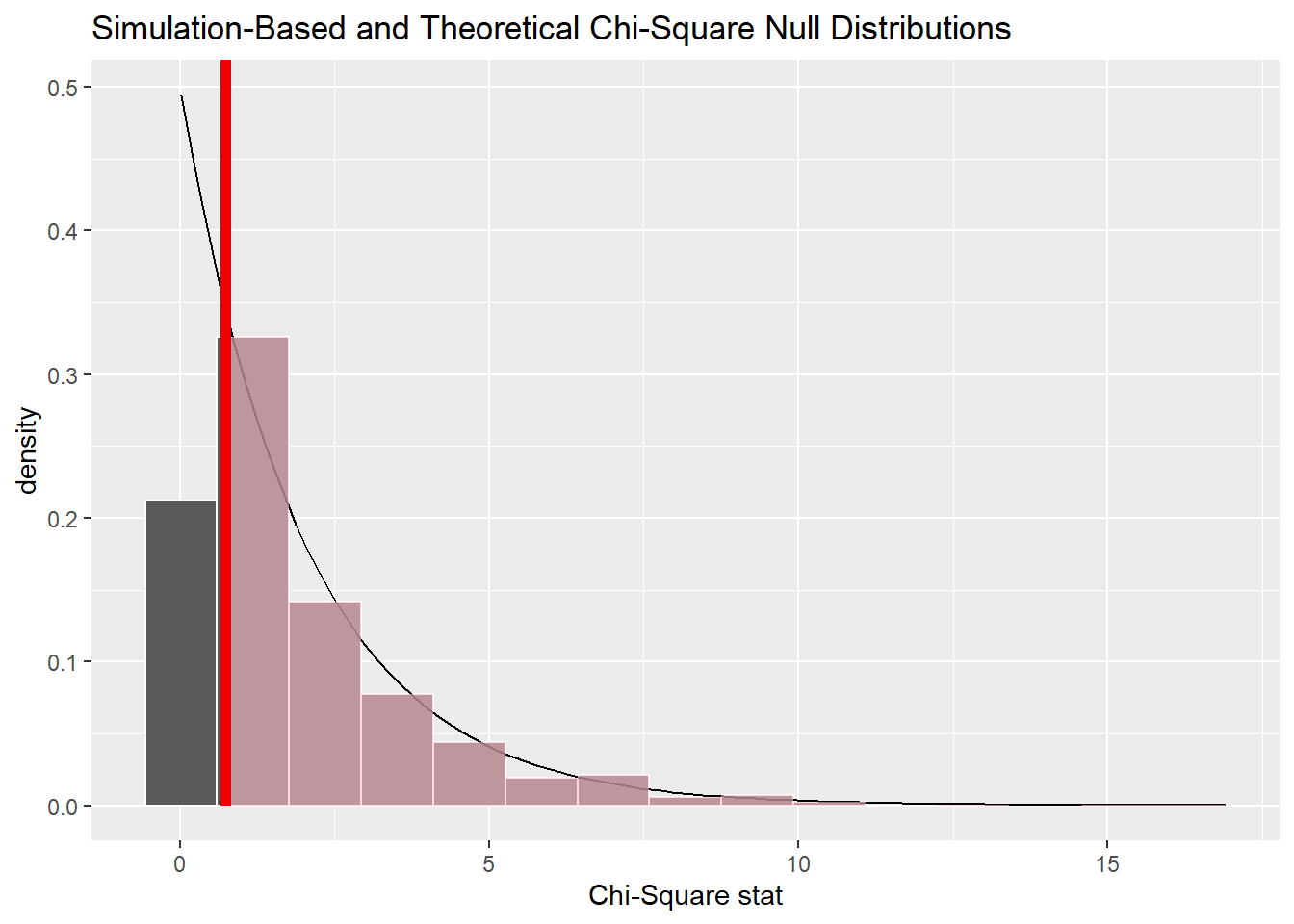
get_p_value(null_chisq, obs_stat = obs_chisq, direction = "greater")# A tibble: 1 × 1
p_value
<dbl>
1 0.7058.10.1 Exact Alternative: Fisher’s Test
Fisher’s test should be considered as an alternative to chi-square when the sample size for some of the classes is small. The usual rule of thumb is that all expected counts should be at least 5, or at least 80% of them should be at least 5 with none below 1. The code below demonstrates this test. Similar to the test above, this test suggests that the difference in proportions or counts in condition classes do not vary between native and non-native trees.
fisher.test(cond_tab, simulate.p.value = TRUE, B = 1e4)
    Fisher's Exact Test for Count Data with simulated p-value (based on
    10000 replicates)

data:  cond_tab
p-value = 0.7167
alternative hypothesis: two.sided
8.10.2 Pairwise Comparisons and CIs for Proportions
We now explore pairwise comparison and confidence intervals when working with proportions. The calculation of confidence intervals using boostrapping and the infer package is demonstrated in the first code block while pairwise comparison is demonstrated in the second. When comparing proportions across more than two groups (e.g., proportion in good condition by functional type), pairwise.prop.test() provides adjusted pairwise comparisons:
    2-sample test for equality of proportions with continuity correction

data:  table(cond_sample$native, cond_sample$good)
X-squared = 4.8103e-31, df = 1, p-value = 1
alternative hypothesis: two.sided
95 percent confidence interval:
 -0.04398265  0.03807159
sample estimates:
    prop 1     prop 2
0.05839416 0.06134969
# Bootstrap CI for the difference in proportions
cond_sample |>
specify(good ~ native, success = "Good") |>
generate(reps = 2000, type = "bootstrap") |>
calculate(stat = "diff in props", order = c("Native", "Non-native")) |>
get_confidence_interval(level = 0.95)# A tibble: 1 × 2
lower_ci upper_ci
<dbl> <dbl>
1 -0.0404 0.0366good_by_type <- trees |>
slice_sample(n = 1000) |>
count(functional_type, good = condition == "Good") |>
pivot_wider(names_from = good, values_from = n, values_fill = 0)
pairwise.prop.test(
x = good_by_type$`TRUE`,
n = good_by_type$`TRUE` + good_by_type$`FALSE`,
p.adjust.method = "holm"
)
    Pairwise comparisons using Pairwise comparison of proportions

data:  good_by_type$`TRUE` out of good_by_type$`TRUE` + good_by_type$`FALSE`

  1 2 3
2 1 - -
3 1 1 -
4 1 1 1

P value adjustment method: holm
8.11 Statistical Power and Sample Size
Power is the probability that a test detects an effect that actually exists (\(1 - \beta\)). Power depends on:
- Effect size: bigger effects are easier to detect
- Sample size: more data reduces the standard error
- Variability: noisier data hides effects
- Significance level \(\alpha\): stricter thresholds lower power
8.11.1 Demo: Type I Error when the Null is True
First, a sanity check. If we shuffle the native labels in the population, there is no true difference. A test at \(\alpha = 0.05\) should reject about 5% of the time.
8.11.2 Demo: Power Curve from Simulation
Now use the real labels, where a true population difference exists. How often do we detect it at different sample sizes? This analysis can be used to determine a required minimum sample size to obtain a desired power.
# A tibble: 2 × 3
  native        mu sigma
  <chr>      <dbl> <dbl>
1 Native      24.9  12.8
2 Non-native  17.6  12.9
power_sim <- expand_grid(n_per_group = c(10, 20, 40, 80, 160, 320)) |>
mutate(power = map_dbl(n_per_group, \(n) {
mean(replicate(500, {
s <- population |> group_by(native) |> slice_sample(n = n) |> ungroup()
t.test(dbh ~ native, data = s)$p.value < 0.05
}))
}))
ggplot(power_sim, aes(n_per_group, power)) +
geom_line() + geom_point(size = 2) +
geom_hline(yintercept = 0.8, linetype = "dashed") +
scale_x_log10() +
labs(x = "Sample size per group (log scale)", y = "Power",
title = "Simulated power to detect the native vs. non-native DBH difference",
subtitle = "Dashed line = conventional 80% power target")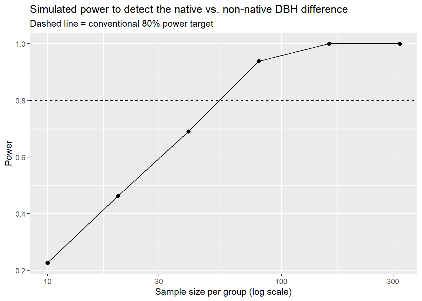
8.11.3 Analytical Power with power.t.test()
For planning studies, base R can solve for any one of n, effect size, \(\alpha\), or power given the others.
     Two-sample t test power calculation

              n = 49.38232
          delta = 7.339589
             sd = 12.88815
      sig.level = 0.05
          power = 0.8
    alternative = two.sided

NOTE: n is number in *each* group
With a large enough sample, trivially small differences become “statistically significant.” Run t.test(dbh ~ native, data = trees) on the full inventory and look at the p-value then look at the confidence interval and ask whether the difference matters to an urban forester. Always report and interpret the effect size and its CI, not just the p-value.
8.12 When Observations Aren’t Independent: Spatial Autocorrelation
Every test in Table 8.1 assumes independent observations. Trees are not scattered at random: trees in the same park were often planted at the same time, of the same species, in the same soil, and are maintained by the same crew. Tobler’s First Law of Geography puts it simply: near things are more related than distant things. This is spatial autocorrelation.
8.12.1 Why it Matters
If neighboring trees are similar, 500 trees from 10 parks contain much less independent information than 500 trees from 500 parks. Standard tests treat each tree as a fresh, independent piece of evidence, so they underestimate standard errors, produce CIs that are too narrow, and produce p-values that are too small. This is sometimes called pseudoreplication.
8.12.2 Demo: See it on a Map
Since these data contain latitude and longitude, we can plot the data in map space and observe a variable across this space. In the example below, we are plotting DBH using a natural log transformation. A simple visual inspection suggests that spatial autocorrelation may be an issue: nearer trees may have more similar DBH.
trees |>
  slice_sample(n = 5000) |>
  ggplot(aes(longitude, latitude, color = log(dbh))) +
  geom_point(size = 0.6, alpha = 0.7) +
  scale_color_viridis_c() +
  coord_quickmap() +
  labs(title = "Park trees in Portland, colored by log(DBH)", color = "log DBH")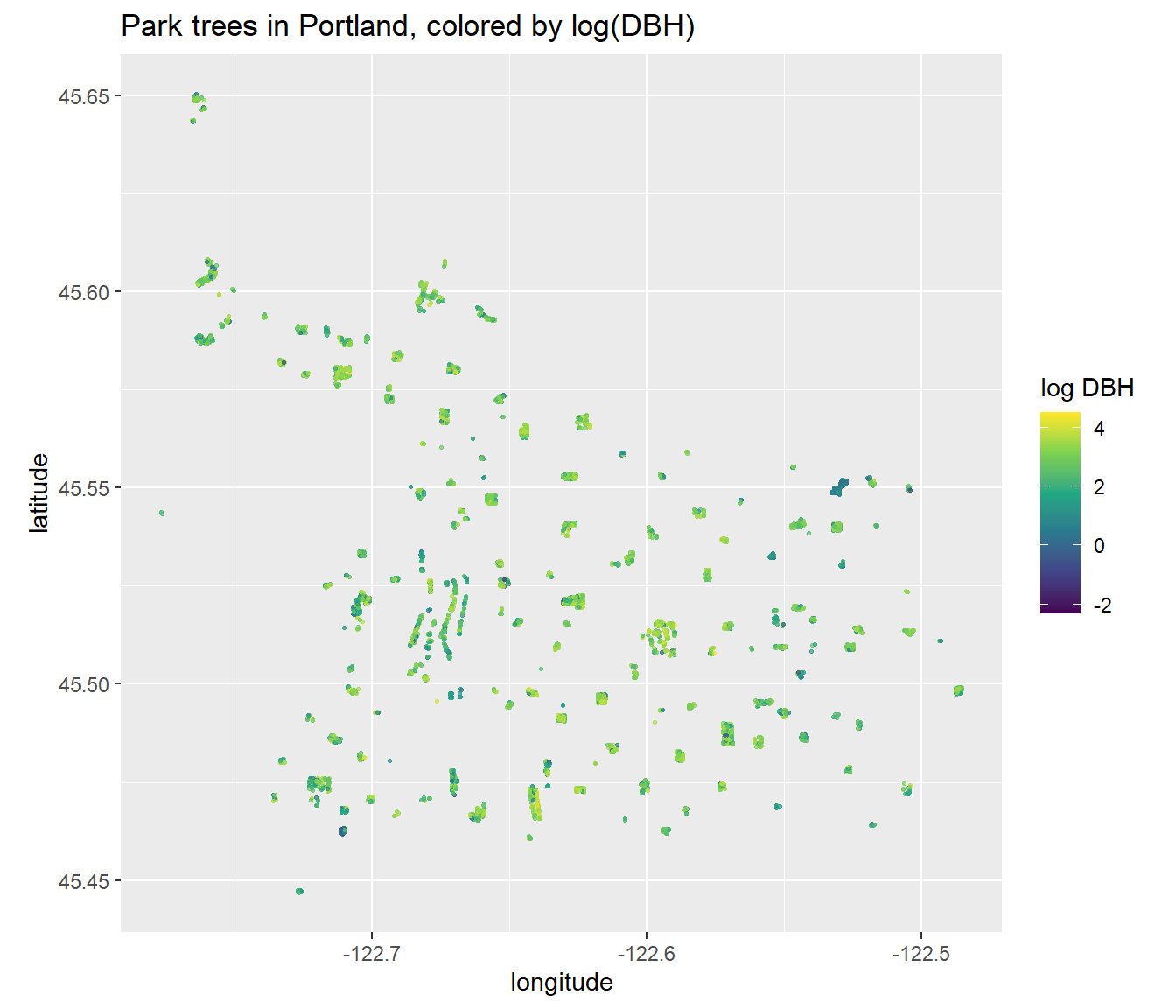
8.12.3 Demo: Measuring it with Moran’s I
Moran’s I measures whether values at nearby locations are more similar (positive I) or more different (negative I) than expected under spatial randomness. We perform this test using the spdep package. We first define who counts as a “neighbor”: here, each tree’s 8 nearest trees. The results below suggest statistical significance. In other words, trees that are closer together tend to have more similar DBH values. In other words, DBH is spatially clustered. Notice that moran.mc() is a permutation test: it shuffles DBH values across locations to see what Moran’s I looks like when space doesn’t matter: exactly the logic we have used with infer.
spatial_sample <- trees |>
  slice_sample(n = 2000) |>
  distinct(longitude, latitude, .keep_all = TRUE)

coords <- as.matrix(spatial_sample[, c("longitude", "latitude")])
nb <- knn2nb(knearneigh(coords, k = 8, longlat = TRUE))
Warning in knn2nb(knearneigh(coords, k = 8, longlat = TRUE)): neighbour object
has 53 sub-graphslw <- nb2listw(nb, style = "W")
# Theory-based test
moran.test(log(spatial_sample$dbh), lw)
    Moran I test under randomisation

data:  log(spatial_sample$dbh)
weights: lw

Moran I statistic standard deviate = 27.832, p-value < 2.2e-16
alternative hypothesis: greater
sample estimates:
Moran I statistic       Expectation          Variance
     0.2910025134     -0.0005002501      0.0001096989
    Monte-Carlo simulation of Moran I

data:  log(spatial_sample$dbh)
weights: lw
number of simulations + 1: 1000

statistic = 0.291, observed rank = 1000, p-value = 0.001
alternative hypothesis: greatertibble(I = moran_mc$res[-length(moran_mc$res)]) |>
ggplot(aes(I)) +
geom_histogram(bins = 40, fill = "grey70", color = "white") +
geom_vline(xintercept = moran_mc$statistic, color = "firebrick", linewidth = 1) +
labs(x = "Moran's I under random spatial arrangement",
title = "Permutation null distribution of Moran's I",
subtitle = "Red line = observed Moran's I")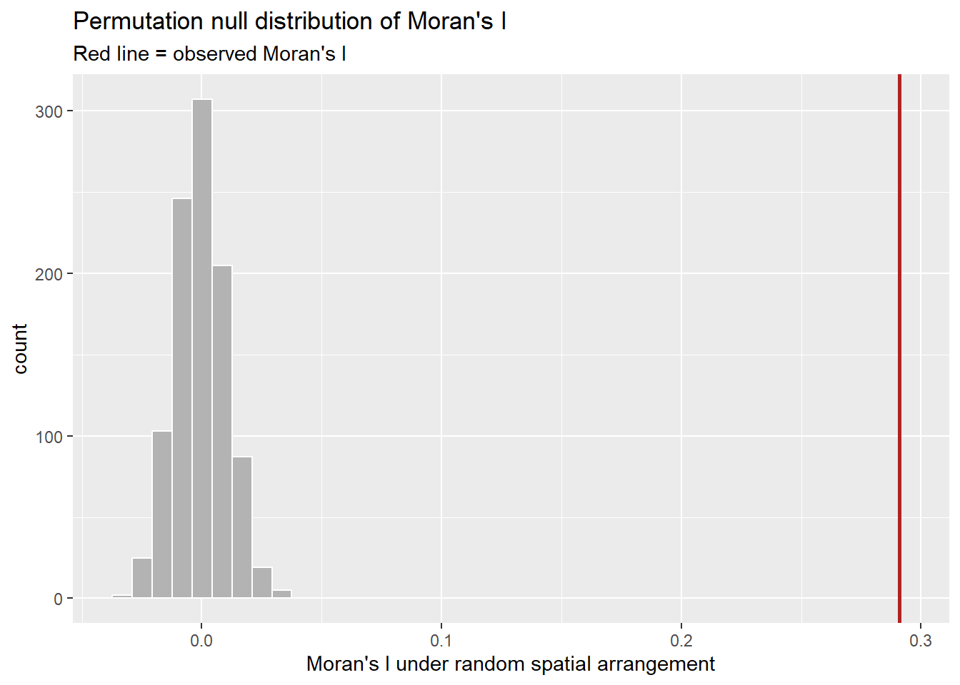
8.12.4 Demo: Clustered Sampling Inflates Uncertainty
Let’s compare two ways to sample 300 trees:
- Simple random sample: 300 trees from anywhere
- Cluster sample: pick 10 parks at random, then 30 trees within each
Both designs use 300 trees, but the cluster sample’s estimates are far more variable. The “naive” standard error, \(s / \sqrt{n}\), which every test in this chapter uses, matches the simple random sample but badly understates the uncertainty of the cluster sample. The ratio of the variances is called the design effect. A design effect of, say, 4 means our 300 clustered trees carry roughly the information of only 75 independent ones: the effective sample size. Here, our design effect for the clustered sample is ~9.
eligible_parks <- trees |> count(park) |> filter(n >= 30) |> pull(park)
trees_elig <- trees |> filter(park %in% eligible_parks)

srs_means <- replicate(1000, mean(slice_sample(trees_elig, n = 300)$dbh))

cluster_means <- replicate(1000, {
  chosen <- sample(eligible_parks, 10)
  trees_elig |>
    filter(park %in% chosen) |>
    group_by(park) |>
    slice_sample(n = 30) |>
    ungroup() |>
    summarize(m = mean(dbh)) |>
    pull(m)
})

sim_compare <- tibble(
  design = rep(c("Simple random sample", "Cluster sample (10 parks x 30)"), each = 1000),
  xbar = c(srs_means, cluster_means)
)

sim_compare |>
  group_by(design) |>
  summarize(true_se = sd(xbar),
            naive_se = sd(trees_elig$dbh) / sqrt(300))
# A tibble: 2 × 3
design true_se naive_se
<chr> <dbl> <dbl>
1 Cluster sample (10 parks x 30) 2.17 0.773
2 Simple random sample 0.745 0.773ggplot(sim_compare, aes(xbar, fill = design)) +
geom_density(alpha = 0.5) +
labs(x = "Sample mean DBH (in)", fill = NULL,
title = "Same sample size, very different uncertainty")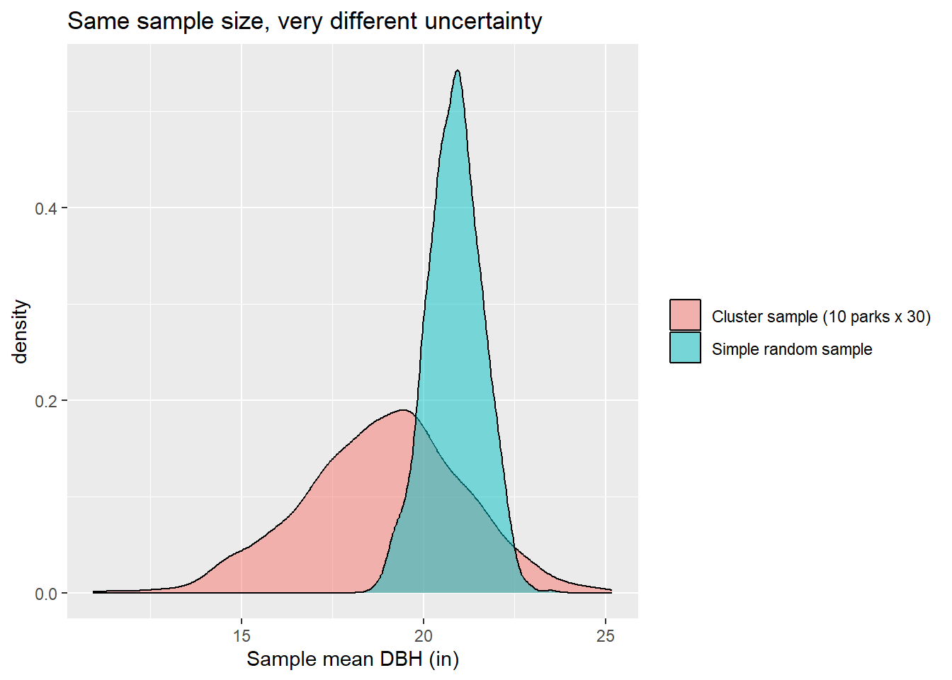
The table below provides some options for dealing with spatial autocorrelation when conducting statistical tests using the Portland trees dataset as an example.
| Strategy | Idea | Tools in R |
|---|---|---|
| Design | Sample randomly across space; space out sampling units | sf::st_sample() |
| Aggregate | Use the cluster (park) as the unit of analysis |
group_by(park) |> summarize() then test |
| Model the structure | Include random effects for clusters | lme4::lmer(dbh ~ native + (1 | park)) |
| Spatial models | Model spatial dependence explicitly |
spatialreg, mgcv::gam(... + s(lon, lat))
|
| Restricted resampling | Permute or bootstrap within blocks, or resample whole blocks | custom group_by() resampling, spatialsample
|
| Diagnose | Test model residuals for leftover autocorrelation | spdep::moran.test(residuals(...), lw) |
As a quick illustration of the aggregation strategy, compare a tree-level test with a park-level test of the same question:
# Tree-level: treats every tree as independent
tree_level <- t.test(dbh ~ native, data = trees_elig) |> tidy() |>
  mutate(level = "Trees as units")

# Park-level: each park contributes one mean per group
park_level <- trees_elig |>
  group_by(park, native) |>
  summarize(dbh = mean(dbh), .groups = "drop") |>
  t.test(dbh ~ native, data = _) |>
  tidy() |>
  mutate(level = "Parks as units")

bind_rows(tree_level, park_level) |>
  select(level, estimate, conf.low, conf.high, p.value)
# A tibble: 2 × 5
level estimate conf.low conf.high p.value
<chr> <dbl> <dbl> <dbl> <dbl>
1 Trees as units 7.30 6.97 7.62 0
2 Parks as units 4.51 2.54 6.47 0.0000101The park-level interval is wider: a more honest reflection of how much independent information we actually have. Note that the two analyses also answer slightly different questions; the mixed model in Table 8.4 reconciles them.
8.13 Concluding Remarks
Here is a summary of the key content discussed in this chapter.
- Inference uses sample statistics to learn about population parameters, and the sampling distribution quantifies how much a statistic varies from sample-to-sample.
- Confidence intervals give a range of plausible values; the “95%” describes the long-run success rate of the method.
- Hypothesis tests compare an observed statistic to a null distribution, which can come from theory (base R:
t.test(),aov(),chisq.test()) or simulation (infer:specify() |> hypothesize() |> generate() |> calculate()). - Nonparametric tests (Wilcoxon, Kruskal–Wallis, Fisher) relax distributional assumptions.
- After an omnibus test, use pairwise comparisons with a multiple-comparison adjustment.
- Power grows with effect size and sample size; with huge samples, focus on effect sizes and CIs, not p-values.
- Spatial autocorrelation violates independence, making naive tests overconfident. Design, aggregate, or model the dependence.
8.14 Questions
- Explain why it does not make sense to use an ANOVA to compare groups when you have data for the entire population.
- Explain the concept of heteroscedasticity.
- Explain the appropriate uses and differences between a one sample t-test, a two sample t-test, and a paired t-test.
- Explain the difference between Type 1 and Type 2 error using an example.
- Explain the concept of statistical power. How is it effected by effect size, sample size, variability, and the chosen significance level.
- Nonparametric statistical tests have no assumptions. Is this statement true or false? Explain you answer.
- What is one pro and one con of using a permutation-based test as opposed to a theory-based test.
- Why is it important to consider effect size even if a statistical test suggests significance?
8.15 Exercises
- Repeat the sampling distribution demo for the median DBH instead of the mean. Is the median’s sampling distribution as well-behaved? How does its standard error compare?
- Build a bootstrap 90% CI for the mean
carbon_storage_lbfrom a sample of 50 trees. Then build a theory-based CI witht.test(). Which is wider, and why might they differ for this variable? - Use a t-test to test whether mean tree height differs between trees in
"Good"condition and all others. Report the test, an effect size, and a 95% CI. Run both a Welch t-test and a permutation test. - Use ANOVA to investigate the following question: do trees with different
mature_size(S, M, L) differ in DBH? Fit an ANOVA, check its assumptions, run Kruskal–Wallis, and perform pairwise comparisons. Write a two-sentence interpretation for a non-statistician. - Using a chi-square test, explore whether
functional_typeis associated withcondition? Inspect expected counts and standardized residuals. Which cells contribute most? - Compute Moran’s I for
tree_height. Then fitlm(log(dbh) ~ native, data = spatial_sample)and test its residuals for spatial autocorrelation. What does this imply about the p-value from that model?