device <- torch_device("cuda")The goal of this article is to provide an example of a complete workflow for a binary classification. We use the topoDL datasets, which consists of historic topographic maps and labels for surface mine disturbance extents. The required data have been provided if you would like to execute the entire workflow. Training this model requires a GPU, and it will take several hours to train the model. We have provided a trained model file if you would like to experiment with the code without training a model from scratch.
Preparation
Since the data have already been provided as chips with associated masks, we do not need to run the makeMasks() and makeChips() processes. Instead, we can start by creating the chip data frames with the makeChipsDF() function. These chips were created outside of the geodl workflow and are stored as .png files as opposed to .tif files, so we have to specify the extension. I am using the “Divided” mode since the positive and background-only chips are stored in separate folders. Note that even though the chips were created outside of the geodl workflow, the folder structure for the directory mimics that created by geodl. So, it is possible to use the makeChipsDF() as long as the folder structure is appropriate. I am also shuffling the chips to reduce autocorrelation. I do not write the chip data frames out to a CSV file.
For this demonstration, I will only use chips that contain at least 1 pixel mapped to the positive case in the training and validation processes, so I use dplyr to filter out only the positive chips. This highlights the value of the included “Division” field. To reduce the training time, I also extract out a random subset of 50% of the chips from the training and validation sets.
trainDF <- makeChipsDF(folder="C:/myFiles/data/topoDL/train/",
extension=".png",
mode="Divided",
shuffle=TRUE,
saveCSV=FALSE)
valDF <- makeChipsDF(folder="C:/myFiles/data/topoDL/val/",
extension=".png",
mode="Divided",
shuffle=TRUE,
saveCSV=FALSE)
trainDF <- trainDF |> filter(division == "Positive") |> sample_frac(.5)
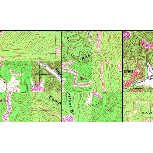
valDF <- valDF |> filter(division == "Positive") |> sample_frac(.5)As a check, I next view a randomly selected set of 25 chips using the viewChips() function.
viewChips(chpDF=trainDF,
          folder="C:/myFiles/data/topoDL/train/",
          nSamps = 25,
          mode = "both",
          justPositive = TRUE,
          cCnt = 5,
          rCnt = 5,
          r = 1,
          g = 2,
          b = 3,
          rescale = FALSE,
          rescaleVal = 1,
          cNames=c("Background", "Mines"),
          cColors=c("gray", "darksalmon"),
          useSeed = TRUE,
          seed = 42)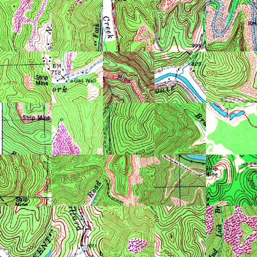
Topo chips examples
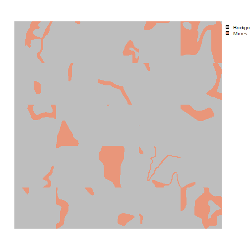
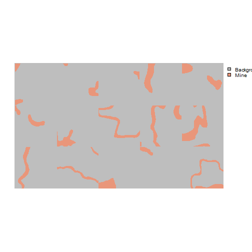
Topo mask chips examples
I am now ready to define the training and validation datasets. Here are a few key points:
- I am not normalizing the data, so do not need to provide band means and standard deviations.
- The topographic map data are scaled from 0 to 255 (8-bit), so I rescale the data from 0 to 1 using a rescaleFactor() of 255. The masks are also scaled from 0 to 255 (0 = background, 255 = mine disturbance), so I rescale the masks from 0 to 1 by setting mskRescale to 255. I also set mskAdd to 1, which will result in the class codes being altered such that 1 = background and 2 = mine disturbance.
Lastly, I apply a maximum of 1 augmentation per chip. The only augmentations used are random vertical and horizontal flips. Both augmentation have a 50% chance of being randomly applied.
I use the same settings for the training and validation datasets other than not applying random augmentations for the validation data.
trainDS <- defineSegDataSet(
  chpDF=trainDF,
  folder="C:/myFiles/data/topoDL/train/",
  normalize = FALSE,
  rescaleFactor = 255,
  mskRescale= 255,
  bands = c(1,2,3),
  mskAdd=1,
  doAugs = TRUE,
  maxAugs = 1,
  probVFlip = .5,
  probHFlip = .5,
  probBrightness = 0,
  probContrast = 0,
  probGamma = 0,
  probHue = 0,
  probSaturation = 0,
  brightFactor = c(.9,1.1),
  contrastFactor = c(.9,1.1),
  gammaFactor = c(.9, 1.1, 1),
  hueFactor = c(-.1, .1),
  saturationFactor = c(.9, 1.1))

valDS <- defineSegDataSet(
  chpDF=valDF,
  folder="C:/myFiles/data/topoDL/val/",
  normalize = FALSE,
  rescaleFactor = 255,
  mskRescale = 255,
  mskAdd=1,
  bands = c(1,2,3),
  doAugs = FALSE,
  maxAugs = 0,
  probVFlip = 0,
  probHFlip = 0)
Next, a print the length of the datasets to make sure the number of samples are as expected.
length(trainDS)
[1] 3886
length(valDS)
[1] 812
Now that I have datasets defined, I generate DataLoaders using the dataloader() function from torch. I use a mini-batch size of 15. You may need to change the mini-batch size depending on your computer’s hardware. The training data are shuffled to reduce autocorrelation; however, the validation data are not. I drop the last mini-batch for both the training and validation data since the last mini-batch may be incomplete.
trainDL <- torch::dataloader(trainDS,
                             batch_size=15,
                             shuffle=TRUE,
                             drop_last = TRUE)

valDL <- torch::dataloader(valDS,
                           batch_size=15,
                           shuffle=FALSE,
                           drop_last = TRUE)
As checks, I next view a batch of the training and validation data using the viewBatch() function. I also use describeBatch() to obtain summary info for a mini-batch. Here are a few points to consider. Note that checks are especially important to conduct in this case since the chips were created outside of the geodl workflow.
- Each mini-batch of images should have a shape of (Mini-Batch, Channels, Width, Height).
- Each mini-batch of masks should have a shape of (Mini-Batch, Class, Width, Height).
- Each image should have a shape of (Channels, Width, Height) and a 32-bit float data type,
- Each mask should have a shape of (Class, Width, Height) and have a long integer data type.
- The number of channels and rows and columns of pixels should match the data being used.
- If you specified a subset of bands, the number of channels should match your subset.
- The range of values in the image bands should be as expected, such as 0 to 1.
- The range of class indices should be as expected. Note whether class codes start at 0 or 1.
- Viewing a mini-batch can help you visualize the augmentations being applied and whether or not they are too extreme or too subtle.
- Viewing the mini-batch can help you determine if there are any oddities with the data, such as the predictor variables and masks not aligning or the bands being in the incorrect order.
viewBatch(dataLoader=trainDL,
          nCols = 5,
          r = 1,
          g = 2,
          b = 3,
          cNames=c("Background", "Mine"),
          cColors=c("gray", "darksalmon")
          )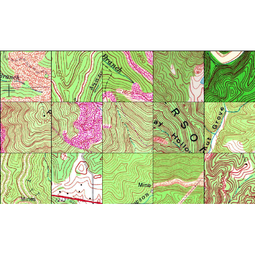
Training chips mini-batch
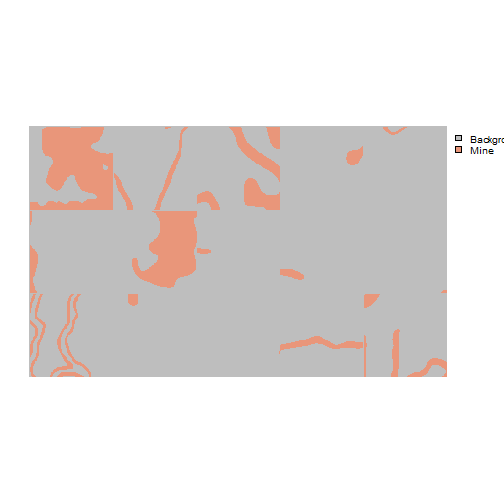
Training masks mini-batch
viewBatch(dataLoader=valDL,
          nCols = 5,
          r = 1,
          g = 2,
          b = 3,
          cNames=c("Background", "Mine"),
          cColors=c("gray", "darksalmon")
          )
Validation chips mini-batch
Validation masks mini-batch
trainStats <- describeBatch(trainDL,
                            zeroStart=FALSE)
valStats <- describeBatch(valDL,
zeroStart=FALSE)print(trainStats)
$batchSize
[1] 15
$imageDataType
[1] "Float"
$maskDataType
[1] "Long"
$imageShape
[1] "15" "3" "256" "256"
$maskShape
[1] "15" "1" "256" "256"
$bndMns
[1] 0.7751913 0.8623868 0.5484013
$bandSDs
[1] 0.1428791 0.1684416 0.2048231
$maskCount
[1] 943233 39807
$minIndex
[1] 1
$maxIndex
[1] 2
print(valStats)
$batchSize
[1] 15
$imageDataType
[1] "Float"
$maskDataType
[1] "Long"
$imageShape
[1] "15" "3" "256" "256"
$maskShape
[1] "15" "1" "256" "256"
$bndMns
[1] 0.7630831 0.8744788 0.5062158
$bandSDs
[1] 0.1316056 0.1597029 0.1757948
$maskCount
[1] 896459 86581
$minIndex
[1] 1
$maxIndex
[1] 2Configure and Train Model with luz
We are now ready to configure and train a model. This is implemented using the luz package, which greatly simplifies the torch training loop. Here are a few key points.
- The UNet model is defined using the defineUNet() function.
- A Tversky loss is implemented with defineUnifiedFocalLoss() by setting lambda to 0, gamma to 1, and delta to 0.6. FN errors will be weighted higher than FP errors.
- We set the zeroStart argument to FALSE since the class codes were set to 1 and 2 using defineSegDataSet().
- As configured, even though this is a binary classification, we are treating it as a multiclass classification, so a logit for the background and positive class will be predicted. This is expected for the loss configuration. All metrics and the UNet model are also configured to expect or generate two class predictions.
- As configured, the assessment metrics (F1-score, precision, and recall) will be calculated using a macro-average of the background and positive cases. If you wanted to only use the positive case, the clsWhgts argument can be changed to c(0,1). clsWghtsDist() in the loss function parameterization can also be changed to c(0,1) so that only the positive case is considered in the loss calculation. However, in this implementation we have chosen to consider both the background and positive case and weight them equally.
- The AdamW optimizer is used.
- The UNet parameterization is configured using set_hparams(). The architecture is configured to generate an output logit for both the positive and background class (nCls = 2). We are using the leaky ReLU activation function (actFunc = “lrelu”) with a negative slope term of 0.01 (negative_slop = 0.01) instead of the more common ReLU. We are using attention gates but not squeeze and excitation modules. We are using the regular bottleneck as opposed to the ASPP module. We are not implementing deep supervision. Encoder blocks 1 through 4 will output 16, 32, 64, and 128 feature maps, respectively. The bottleneck will generate 256 feature maps. Decoder blocks 1 through 4 will output 128, 64, 32, and 16 feature maps, respectively.
- The learning rate is set to 1e-3 using the set_opt_hparams() function from luz.
- Using fit() from luz, we specify the training (data) and validation (valid_data) DataLoaders to use. We train the model for 10 epochs, save the logs out to disk as a CSV file, and only save the model checkpoint if the validation loss improves. We also specify that the GPU will be used for training.
Again, if you want to run this code, expect it to take several hours. A CUDA-enabled GPU is required.
model <- defineUNet |>
  luz::setup(
    loss = defineUnifiedFocalLoss(nCls=2,
                                lambda=0,
                                gamma=1,
                                delta=0.6,
                                smooth = 1e-8,
                                zeroStart=FALSE,
                                clsWghtsDist=1,
                                clsWghtsReg=1,
                                useLogCosH =FALSE,
                                device="cuda"),
    optimizer = optim_adamw,
    metrics = list(
      luz_metric_overall_accuracy(nCls=2,
                                  smooth=1,
                                  mode = "multiclass",
                                  zeroStart= FALSE,
                                  usedDS = FALSE),
      luz_metric_f1score(nCls=2,
                         smooth=1,
                         mode = "multiclass",
                         zeroStart= FALSE,
                         clsWghts=c(1,1),
                         usedDS = FALSE),
      luz_metric_recall(nCls=2,
                        smooth=1,
                        mode = "multiclass",
                        zeroStart= FALSE,
                        clsWghts=c(1,1),
                        usedDS = FALSE),
      luz_metric_precision(nCls=2,
                           smooth=1,
                           mode = "multiclass",
                           zeroStart= FALSE,
                           clsWghts=c(1,1),
                           usedDS = FALSE)
    )
  ) |>
  set_hparams(inChn = 3,
              nCls = 2,
              actFunc = "lrelu",
              useAttn = TRUE,
              useSE = FALSE,
              useRes = FALSE,
              useASPP = FALSE,
              useDS = FALSE,
              enChn = c(16,32,64,128),
              dcChn = c(128,64,32,16),
              btnChn = 256,
              dilRates=c(1,2,4,8,16),
              dilChn=c(16,16,16,16,16),
              negative_slope = 0.01,
              seRatio=8) |>
  set_opt_hparams(lr = 1e-3) |>
  fit(data=trainDL,
      valid_data=valDL,
      epochs = 10,
      callbacks = list(luz_callback_csv_logger("C:/myFiles/data/topoDL/models/trainLogs.csv"),
                       luz_callback_model_checkpoint(path="data/topoDL/models/",
                                                     monitor="valid_loss",
                                                     save_best_only=TRUE,
                                                     mode="min",
                       )),
      accelerator = accelerator(device_placement = TRUE,
                                cpu = FALSE,
                                cuda_index = torch::cuda_current_device()),
      verbose=TRUE)
Assess Model
Once the model is trained, it should be assessed using the withheld testing set. To accomplish this, we first re-instantiate the model using luz and by loading the saved checkpoint. In fit(), we set the argument for epoch to 0 so that the model object is instantiated but no training is conducted. We then load the saved checkpoint using luz_load_checkpoint().
model <- defineUNet |>
  luz::setup(
    loss = defineUnifiedFocalLoss(nCls=2,
                                  lambda=0,
                                  gamma=1,
                                  delta=0.6,
                                  smooth = 1e-8,
                                  zeroStart=FALSE,
                                  clsWghtsDist=1,
                                  clsWghtsReg=1,
                                  useLogCosH =FALSE,
                                  device="cuda"),
    optimizer = optim_adamw,
    metrics = list(
      luz_metric_overall_accuracy(nCls=2,
                                  smooth=1,
                                  mode = "multiclass",
                                  zeroStart= FALSE,
                                  usedDS = FALSE),
      luz_metric_f1score(nCls=2,
                         smooth=1,
                         mode = "multiclass",
                         zeroStart= FALSE,
                         clsWghts=c(1,1),
                         usedDS = FALSE),
      luz_metric_recall(nCls=2,
                        smooth=1,
                        mode = "multiclass",
                        zeroStart= FALSE,
                        clsWghts=c(1,1),
                        usedDS = FALSE),
      luz_metric_precision(nCls=2,
                           smooth=1,
                           mode = "multiclass",
                           zeroStart= FALSE,
                           clsWghts=c(1,1),
                           usedDS = FALSE)
    )
  ) |>
  set_hparams(inChn = 3,
              nCls = 2,
              actFunc = "lrelu",
              useAttn = TRUE,
              useSE = FALSE,
              useRes = FALSE,
              useASPP = FALSE,
              useDS = FALSE,
              enChn = c(16,32,64,128),
              dcChn = c(128,64,32,16),
              btnChn = 256,
              dilRates=c(1,2,4,8,16),
              dilChn=c(16,16,16,16,16),
              negative_slope = 0.01,
              seRatio=8) |>
  set_opt_hparams(lr = 1e-3) |>
  fit(data=trainDL,
      valid_data=valDL,
      epochs = 0,
      callbacks = list(luz_callback_csv_logger("C:/myFiles/data/topoDL/models/trainLogs.csv"),
                       luz_callback_model_checkpoint(path="data/topoDL/models/",
                                                     monitor="valid_loss",
                                                     save_best_only=TRUE,
                                                     mode="min",
                       )),
      accelerator = accelerator(device_placement = TRUE,
                                cpu = FALSE,
                                cuda_index = torch::cuda_current_device()),
      verbose=TRUE)
luz_load_checkpoint(model, "C:/myFiles/data/topoDL/topoDLModel.pt")We read in the saved logs from disk and plot the training and validation loss, F1-score, recall, and precision curves using ggplot2.
allMets <- read.csv("C:/myFiles/data/topoDL/trainLogs.csv")
ggplot(allMets, aes(x=epoch, y=loss, color=set))+
  geom_line(lwd=1)+
  labs(x="Epoch", y="Loss", color="Set")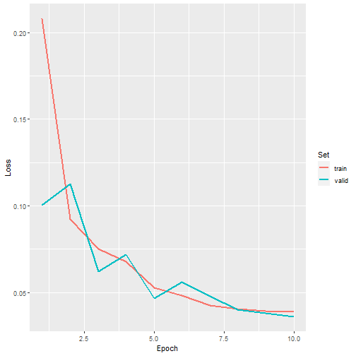
Loss graph
ggplot(allMets, aes(x=epoch, y=f1score, color=set))+
  geom_line(lwd=1)+
  labs(x="Epoch", y="F1-Score", color="Set")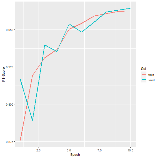
F1-score graph
ggplot(allMets, aes(x=epoch, y=recall, color=set))+
  geom_line(lwd=1)+
  labs(x="Epoch", y="Recall", color="Set")
Recall graph
ggplot(allMets, aes(x=epoch, y=precision, color=set))+
  geom_line(lwd=1)+
  labs(x="Epoch", y="Precision", color="Set")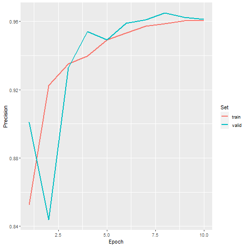
Precision graph
Next, we load in the test data. This requires (1) listing the chips into a data frame using makeChipsDF(), (2) defining a DataSet using defineSegDataset(), and (3) creating a DataLoader with torch::dataloader(). It is important that the dataset is defined to be consistent with the training and validation datasets used to train and validate the model during the training process.
testDF <- makeChipsDF(folder="C:/myFiles/data/topoDL/test/",
                     extension=".png",
                     mode="Divided",
                     shuffle=TRUE,
                     saveCSV=FALSE) |> filter(division=="Positive")
testDS <- defineSegDataSet(
  chpDF=testDF,
  folder="C:/myFiles/data/topoDL/test/",
  normalize = FALSE,
  rescaleFactor = 255,
  mskRescale = 255,
  mskAdd=1,
  bands = c(1,2,3),
  doAugs = FALSE,
  maxAugs = 0,
  probVFlip = 0,
  probHFlip = 0)
testDL <- torch::dataloader(testDS,
                           batch_size=15,
                           shuffle=FALSE,
                           drop_last = TRUE)
We can obtain the same summary metrics as used during the training process but calculated for the withheld testing data using the evaluate() function from luz. Once the evaluation is ran, the metrics can be obtained with get_metrics().
testEval <- model %>% evaluate(data=testDL)
assMets <- get_metrics(testEval)
print(assMets)
# A tibble: 5 × 2
  metric      value
  <chr>       <dbl>
1 loss       0.0286
2 overallacc 0.987
3 f1score    0.973
4 recall     0.977
5 precision  0.969
Using geodl, a mini-batch of topographic map chips, reference masks, and predictions can be plotted using viewBatchPreds(). Summary metrics can be obtain for the entire training dataset using assessDL() from geodl. This function generates the same set of metrics as assessPnts() and assessRaster()
viewBatchPreds(dataLoader=testDL,
               model=model,
               mode="multiclass",
               nCols =5,
               r = 1,
               g = 2,
               b = 3,
               cCodes=c(1,2),
               cNames=c("Not Mine", "Mine"),
               cColors=c("gray", "darksalmon"),
               useCUDA=TRUE,
               probs=FALSE,
               usedDS=FALSE)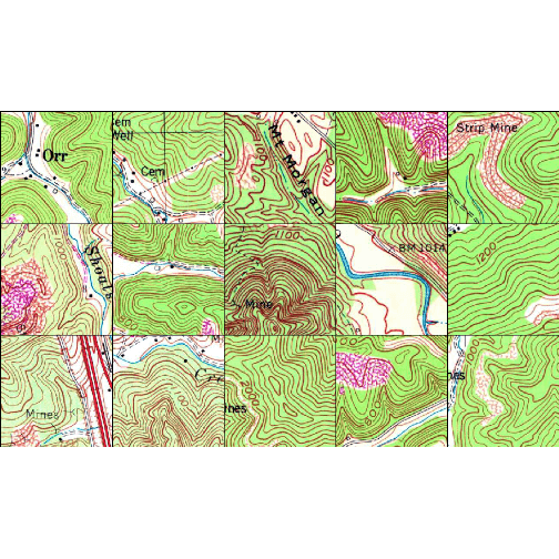
Chips to predict

Reference masks
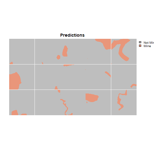
Predictions
metricsOut <- assessDL(dl=testDL,
                       model=model,
                       batchSize=15,
                       size=256,
                       nCls=2,
                       multiclass=FALSE,
                       cCodes=c(1,2),
                       cNames=c("Not Mine", "Mine"),
                       usedDS=FALSE,
                       useCUDA=TRUE,
decimals=4)print(metricsOut)
$Classes
[1] "Not Mine" "Mine"
$referenceCounts
Negative Positive
70304626 11287694
$predictionCounts
Negative Positive
70086175 11506145
$ConfusionMatrix
Reference
Predicted Negative Positive
Negative 69669489 416686
Positive 635137 10871008
$Mets
OA Recall Precision Specificity NPV F1Score
Mine 0.9871 0.9631 0.9448 0.991 0.9941 0.9539This is an example of an entire workflow to train and validate a deep learning semantic segmentation model to extract surface mine disturbance extents from historic topographic maps using geodl. We also made use of luz to implement the training loop. This example serves as a good starting point to build a training and validation pipeline for your own custom dataset.