device <- torch_device("cuda")The goal of this article is to provide an example of a complete workflow for a multiclass classification. We use the landcover.ai datasets, which consists of high spatial resolution aerial orthophotography for areas across Poland. The associated labels differentiate five classes: Background, Buildings, Woodland, Water, and Road. The required data have been provided if you would like to execute the entire workflow. Training this model requires a GPU, and it will take several hours to train the model. We have provided a trained model file if you would like to experiment with the code without training a model from scratch.
Preparation
The data originators have provides TXT files listing the image chips into separate training, validation, and testing datasets. So, we first read in these lists as data frames. The data lists are not in the correct format for geodl’s defineSegDataset() function, which requires that the following columns are present: “chpN”, “chpPth”, and “mskPth”. The “chpN” column must provides the name of the chip, and the “chpPth” and “MskPth” columns must provide the path to the image and associated mask chips relative to the folder that houses the chips. Using dplyr, we create data frames in this correct format from the provided tables. The mask files have the suffix “_m” added, so we also must add this suffix to the image name when defining the associated mask.
Lastly, we randomly select out 3,000 training, 500 validation, and 500 testing chips to speed up the training and inference processes for this demonstration.
testDF <- read.csv("C:/myFiles/data/landcoverai/test.txt", header=FALSE)
trainDF <- read.csv("C:/myFiles/data/landcoverai/train.txt", header=FALSE)
valDF <-  read.csv("C:/myFiles/data/landcoverai/val.txt", header=FALSE)
trainDF <- data.frame(chpN=trainDF$V1,
chpPth=paste0("images/", trainDF$V1, ".tif"),
mskPth=paste0("masks/", trainDF$V1, "_m.tif")) |>
sample_frac(1, replace=FALSE) |> sample_n(3000)
testDF <- data.frame(chpN=testDF$V1,
chpPth=paste0("images/", testDF$V1, ".tif"),
mskPth=paste0("masks/", testDF$V1, "_m.tif")) |>
sample_frac(1, replace=FALSE) |> sample_n(500)
valDF <- data.frame(chpN=valDF$V1,
chpPth=paste0("images/", valDF$V1, ".tif"),
mskPth=paste0("masks/", valDF$V1, "_m.tif")) |>
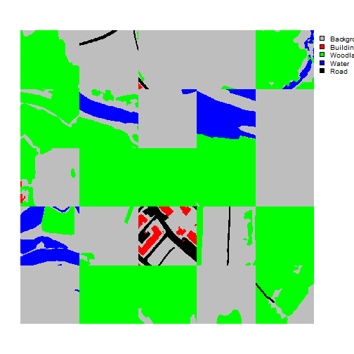
sample_frac(1, replace=FALSE) |> sample_n(500)As a check, I next view a randomly selected set of 25 chips using the viewChips() function.
viewChips(chpDF=trainDF,
          folder="C:/myFiles/data/landcoverai/train/",
          nSamps = 25,
          mode = "both",
          justPositive = FALSE,
          cCnt = 5,
          rCnt = 5,
          r = 1,
          g = 2,
          b = 3,
          rescale = FALSE,
          rescaleVal = 1,
          cNames= c("Background", "Buildings", "Woodland", "Water", "Road"),
          cColors= c("gray", "red", "green", "blue", "black"),
          useSeed = TRUE,
          seed = 42)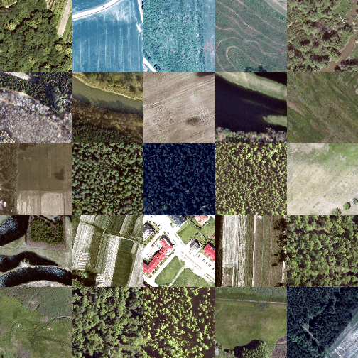
I am now ready to define the training and validation datasets. Here are a few key points:
- I am not normalizing the data, so do not need to provide band means and standard deviations.
- The images are scaled from 0 to 255 (8-bit), so I rescale the data from 0 to 1 using a rescaleFactor() of 255. The masks do not need to be rescaled. I also set mskAdd to 1 so that the class codes will begin at 1 instead of 0.
- Lastly, I apply a maximum of 1 augmentation per chip. The augmentations used are random vertical flips, horizontal flips, brightness changes, and saturation changes. Horizontal and vertical flips have a 50% chance of being randomly applied, brightness changes have a 10% chance of being applied, and saturation changes have a 20% chance of being applied.
I use the same settings for the training and validation datasets other than not applying random augmentations for the validation data.
trainDS <- defineSegDataSet(
  chpDF=trainDF,
  folder="C:/myFiles/data/landcoverai/train/",
  normalize = FALSE,
  rescaleFactor = 255,
  mskRescale= 1,
  bands = c(1,2,3),
  mskAdd=1,
  doAugs = TRUE,
  maxAugs = 1,
  probVFlip = .5,
  probHFlip = .5,
  probBrightness = .1,
  probContrast = 0,
  probGamma = 0,
  probHue = 0,
  probSaturation = .2,
  brightFactor = c(.9,1.1),
  contrastFactor = c(.9,1.1),
  gammaFactor = c(.9, 1.1, 1),
  hueFactor = c(-.1, .1),
  saturationFactor = c(.9, 1.1))

valDS <- defineSegDataSet(
  chpDF=valDF,
  folder="C:/myFiles/data/landcoverai/val/",
  normalize = FALSE,
  rescaleFactor = 255,
  mskRescale = 1,
  mskAdd=1,
  bands = c(1,2,3),
  doAugs = FALSE,
  maxAugs = 0,
  probVFlip = 0,
  probHFlip = 0)
Next, a print the length of the datasets to make sure the number of samples are as expected.
length(trainDS)
[1] 3000
length(valDS)
[1] 500
Now that I have datasets defined, I generate DataLoaders using the dataloader() function from torch. I use a mini-batch size of 15. You may need to change the mini-batch size depending on your computer’s hardware. The training data are shuffled to reduce autocorrelation; however, the validation data are not. I drop the last mini-batch for both the training and validation data.
trainDL <- torch::dataloader(trainDS,
batch_size=15,
shuffle=TRUE,
drop_last = TRUE)
valDL <- torch::dataloader(valDS,
batch_size=15,
shuffle=FALSE,
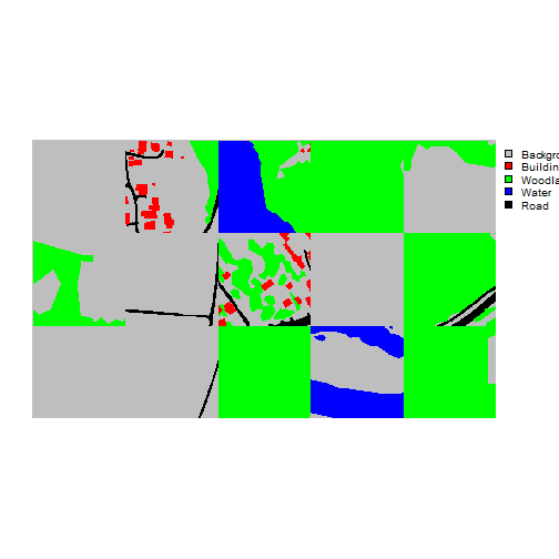
drop_last = TRUE)As checks, I next view a batch of the training and validation data using the viewBatch() function. I also use describeBatch() to obtain summary info for a mini-batch. Here are a few points to consider.
- Each mini-batch of images should have a shape of (Mini-Batch, Channels, Width, Height).
- Each mini-batch of masks should have a shape of (Mini-Batch, Class, Width, Height).
- Each image should have a shape of (Channels, Width, Height) and a 32-bit float data type,
- Each mask should have a shape of (Class, Width, Height) and have a long integer data type.
- The number of channels and rows and columns of pixels should match the data being used.
- If you specified a subset of bands, the number of channels should match your subset.
- The range of values in the image bands should be as expected, such as 0 to 1.
- The range of class indices should be as expected. Note whether class codes start at 0 or 1.
- Viewing a mini-batch can help you visualize the augmentations being applied and whether or not they are too extreme or too subtle.
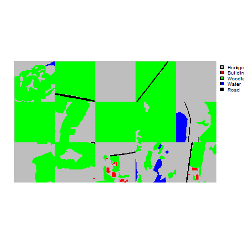
- Viewing the mini-batch can help you determine if there are any oddities with the data, such as the predictor variables and masks not aligning or the bands being in the incorrect order.
viewBatch(dataLoader=trainDL,
          nCols = 5,
          r = 1,
          g = 2,
          b = 3,
          cNames=c("Background", "Buildings", "Woodland", "Water", "Road"),
          cColors=c("gray", "red", "green", "blue", "black"))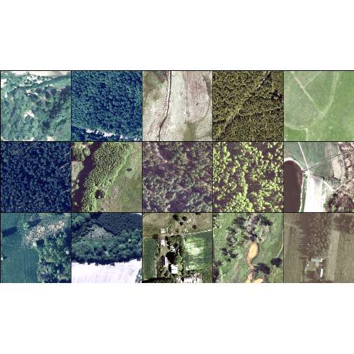
viewBatch(dataLoader=valDL,
          nCols = 5,
          r = 1,
          g = 2,
          b = 3,
          cNames=c("Background", "Buildings", "Woodland", "Water", "Road"),
          cColors=c("gray", "red", "green", "blue", "black"))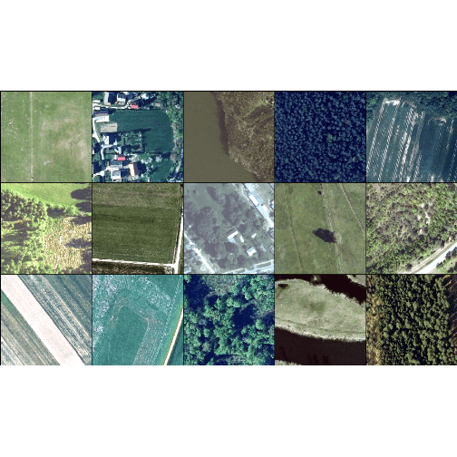
trainStats <- describeBatch(trainDL,
                            zeroStart=FALSE)
valStats <- describeBatch(valDL,
zeroStart=FALSE)print(trainStats)
$batchSize
[1] 15
$imageDataType
[1] "Float"
$maskDataType
[1] "Long"
$imageShape
[1] "15" "3" "512" "512"
$maskShape
[1] "15" "1" "512" "512"
$bndMns
[1] 0.3979441 0.4192438 0.3617396
$bandSDs
[1] 0.1630734 0.1325573 0.1078829
$maskCount
[1] 2618263 14723 1063879 15848 219447
$minIndex
[1] 1
$maxIndex
[1] 5
print(valStats)
$batchSize
[1] 15
$imageDataType
[1] "Float"
$maskDataType
[1] "Long"
$imageShape
[1] "15" "3" "512" "512"
$maskShape
[1] "15" "1" "512" "512"
$bndMns
[1] 0.3086319 0.3634965 0.3161972
$bandSDs
[1] 0.1500528 0.1296813 0.1046080
$maskCount
[1] 2183194 53566 1374415 259548 61437
$minIndex
[1] 1
$maxIndex
[1] 5Configure and Train Model with luz
We are now ready to configure and train a model. This is implemented using the luz package, which greatly simplifies the torch training loop. Here are a few key points.
- A UNet model with a MobileNet-v2 encoder is defined using the defineMobileUNet() function. Note that this implementation only accepts three-band inputs data.
- A focal Dice loss is implemented with defineUnifiedFocalLoss() by setting lambda to 0, gamma to 0.8, and delta to 0.5.
- We set the zeroStart argument to FALSE since the class codes were set start at 1 using defineSegDataSet().
- The loss metric and all assessment metrics are configured to expect 5 classes.
- The AdamW optimizer is used.
- The UNet parameterization is configured using set_hparams(). The architecture is configured to generate an output logit for all 5 classes (nCls = 5). We are using the leaky ReLU activation function (actFunc = “lrelu”) with a negative slope term of 0.01 (negative_slop = 0.01) instead of the more common ReLU. We are using attention gates but not deep supervision. Decoder blocks 1 through 5 will output 256, 128, 64, 32, and 16 feature maps, respectively.
- The learning rate is set to 1e-3 using the set_opt_hparams() function from luz.
- Using fit() from luz, we specify the training (data) and validation (valid_data) DataLoaders to use. We train the model for 10 epochs, save the logs out to disk as a CSV file, and only save the model checkpoint if the validation loss improves. We also specify that the GPU will be used for training.
Again, if you want to run this code, expect it to take several hours. A CUDA-enabled GPU is required.
fitted <- defineMobileUNet |>
  luz::setup(
    loss = defineUnifiedFocalLoss(nCls=5,
                                    lambda=0,
                                    gamma=.8,
                                    delta=0.5,
                                    smooth = 1,
                                    zeroStart=FALSE,
                                    clsWghtsDist=1,
                                    clsWghtsReg=1,
                                    useLogCosH =FALSE,
                                    device=device),
    optimizer = optim_adamw,
    metrics = list(
      luz_metric_overall_accuracy(nCls=5,
                                  smooth=1,
                                  mode="multiclass",
                                  zeroStart=FALSE,
                                  usedDS=FALSE),
      luz_metric_f1score(nCls=5,
                         smooth=1,
                         mode="multiclass",
                         zeroStart=FALSE,
                         clsWghts=c(1,1,1,1,1),
                         usedDS=FALSE),
      luz_metric_recall(nCls=5,
                         smooth=1,
                         mode="multiclass",
                         zeroStart=FALSE,
                        clsWghts=c(1,1,1,1,1),
                         usedDS=FALSE),
      luz_metric_precision(nCls=5,
                         smooth=1,
                         mode="multiclass",
                         zeroStart=FALSE,
                         clsWghts=c(1,1,1,1,1),
                         usedDS=FALSE)
    )
  ) |>
  set_hparams(
    nCls = 5,
    pretrainedEncoder = TRUE,
    freezeEncoder = FALSE,
    actFunc = "lrelu",
    useAttn = TRUE,
    useDS = FALSE,
    dcChn = c(256,128,64,32,16),
    negative_slope = 0.01
  ) |>
  set_opt_hparams(lr = 1e-3) |>
  fit(data=trainDL,
      valid_data=valDL,
      epochs = 10,
      callbacks = list(luz_callback_csv_logger("C:/myFiles/data/landcoverai/models/trainLogs.csv"),
                       luz_callback_model_checkpoint(path="data/landcoverai/models/",
                                                     monitor="valid_loss",
                                                     save_best_only=TRUE,
                                                     mode="min",
                       )),
      accelerator = accelerator(device_placement = TRUE,
                                cpu = FALSE,
                                cuda_index = torch::cuda_current_device()),
      verbose=TRUE)
Assess Model
Once the model is trained, it should be assessed using the withheld testing set. To accomplish this, we first re-instantiate the model using luz and by loading the saved checkpoint. In fit(), we set the argument for epoch to 0 so that the model object is instantiated but no training is conducted. We then load the saved checkpoint using luz_load_checkpoint().
fitted <- defineMobileUNet |>
  luz::setup(
    loss = defineUnifiedFocalLoss(nCls=5,
                                  lambda=0,
                                  gamma=.8,
                                  delta=0.5,
                                  smooth = 1,
                                  zeroStart=FALSE,
                                  clsWghtsDist=1,
                                  clsWghtsReg=1,
                                  useLogCosH =FALSE,
                                  device=device),
    optimizer = optim_adamw,
    metrics = list(
      luz_metric_overall_accuracy(nCls=5,
                                  smooth=1,
                                  mode="multiclass",
                                  zeroStart=FALSE,
                                  usedDS=FALSE),
      luz_metric_f1score(nCls=5,
                         smooth=1,
                         mode="multiclass",
                         zeroStart=FALSE,
                         clsWghts=c(1,1,1,1,1),
                         usedDS=FALSE),
      luz_metric_recall(nCls=5,
                        smooth=1,
                        mode="multiclass",
                        zeroStart=FALSE,
                        clsWghts=c(1,1,1,1,1),
                        usedDS=FALSE),
      luz_metric_precision(nCls=5,
                           smooth=1,
                           mode="multiclass",
                           zeroStart=FALSE,
                           clsWghts=c(1,1,1,1,1),
                           usedDS=FALSE)
    )
  ) |>
  set_hparams(
    nCls = 5,
    pretrainedEncoder = TRUE,
    freezeEncoder = FALSE,
    actFunc = "lrelu",
    useAttn = FALSE,
    useDS = FALSE,
    dcChn = c(256,128,64,32,16),
    negative_slope = 0.01
  ) |>
  set_opt_hparams(lr = 1e-3) |>
  fit(data=trainDL,
      valid_data=valDL,
      epochs = 0,
      callbacks = list(luz_callback_csv_logger("C:/myFiles/data/landcoverai/models/trainLogs.csv"),
                       luz_callback_model_checkpoint(path="data/landcoverai/models/",
                                                     monitor="valid_loss",
                                                     save_best_only=TRUE,
                                                     mode="min",
                       )),
      accelerator = accelerator(device_placement = TRUE,
                                cpu = FALSE,
                                cuda_index = torch::cuda_current_device()),
      verbose=TRUE)
luz_load_checkpoint(fitted, "C:/myFiles/data/landcoverai/landcoveraiModel.pt")We read in the saved logs from disk and plot the training and validation loss, F1-score, recall, and precision curves using ggplot2.
allMets <- read.csv("C:/myFiles/data/landcoverai/trainLogs.csv")
ggplot(allMets, aes(x=epoch, y=loss, color=set))+
  geom_line(lwd=1)+
  labs(x="Epoch", y="Loss", color="Set")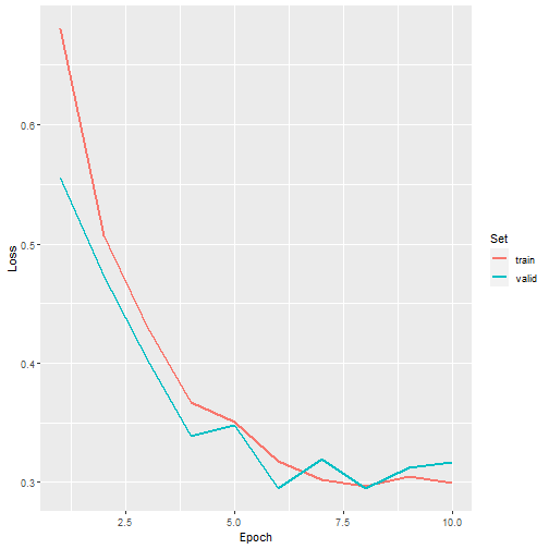
Loss graph
ggplot(allMets, aes(x=epoch, y=f1score, color=set))+
  geom_line(lwd=1)+
  labs(x="Epoch", y="F1-Score", color="Set")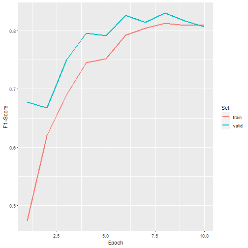
F1-score graph
ggplot(allMets, aes(x=epoch, y=recall, color=set))+
  geom_line(lwd=1)+
  labs(x="Epoch", y="Recall", color="Set")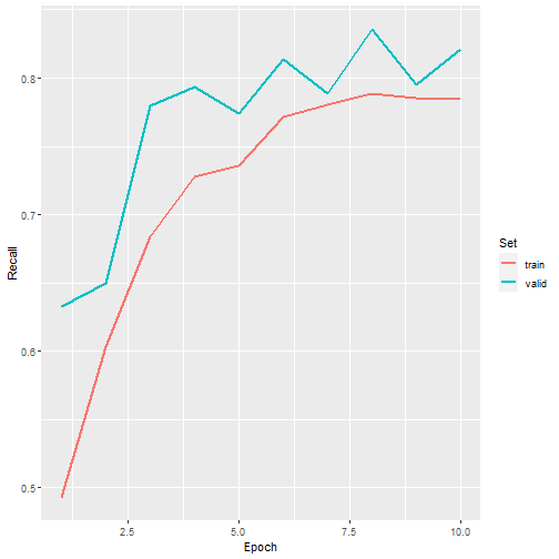
Recall graph
ggplot(allMets, aes(x=epoch, y=precision, color=set))+
  geom_line(lwd=1)+
  labs(x="Epoch", y="Precision", color="Set")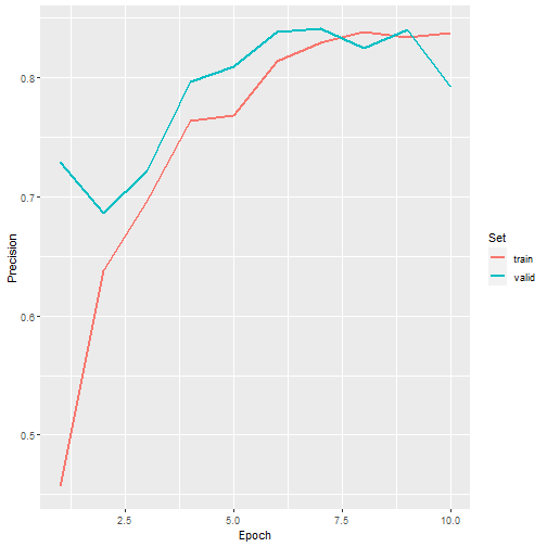
Precision graph
Next, we load in the test data. This requires (1) listing the chips into a data frame using makeChipsDF() (this was already done above), (2) defining a DataSet using defineSegDataset(), and (3) creating a DataLoader with torch::dataloader(). It is important that the dataset is defined to be consistent with the training and validation datasets used to train and validate the model during the training process.
testDS <- defineSegDataSet(
  chpDF=testDF,
  folder="C:/myFiles/data/landcoverai/test/",
  normalize = FALSE,
  rescaleFactor = 255,
  mskRescale = 1,
  mskAdd=1,
  bands = c(1,2,3),
  doAugs = FALSE,
  maxAugs = 0,
  probVFlip = 0,
  probHFlip = 0)
testDL <- torch::dataloader(testDS,
                           batch_size=15,
                           shuffle=FALSE,
                           drop_last = TRUE)
We can obtain the same summary metrics as used during the training process but calculated for the withheld testing data using the evaluate() function from luz. Once the evaluation is ran, the metrics can be obtained with get_metrics().
testEval <- fitted %>% evaluate(data=testDL)
assMets <- get_metrics(testEval)
print(assMets)
# A tibble: 5 × 2
metric value
<chr> <dbl>
1 loss 0.261
2 overallacc 0.924
3 f1score 0.837
4 recall 0.818
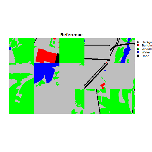
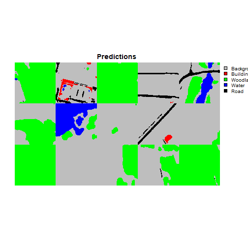
5 precision 0.858Using geodl, a mini-batch of image chips, reference masks, and predictions can be plotted using viewBatchPreds(). Summary metrics can be obtain for the entire training dataset using assessDL() from geodl. This function generates the same set of metrics as assessPnts() and assessRaster()
viewBatchPreds(dataLoader=testDL,
               model=fitted,
               mode="multiclass",
               nCols = 5,
               r = 1,
               g = 2,
               b = 3,
               cCodes=c(1,2,3,4,5),
               cNames=c("Background", "Buildings", "Woodland", "Water", "Road"),
               cColors=c("gray", "red", "green", "blue", "black"),
               useCUDA=TRUE,
               probs=FALSE,
               usedDS=FALSE)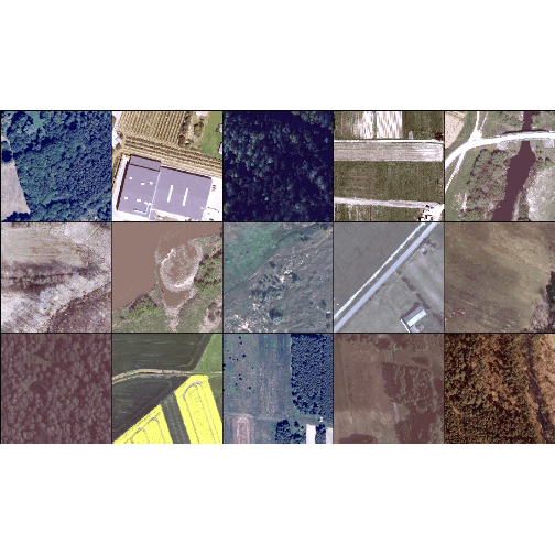
testEval2 <- assessDL(dl=testDL,
                      model=fitted,
                      batchSize=12,
                      size=512,
                      nCls=5,
                      multiclass=TRUE,
                      cCodes=c(1,2,3,4,5),
                      cNames=c("Background", "Buildings", "Woodland", "water", "road"),
                      usedDS=FALSE,
useCUDA=TRUE)print(testEval2)
$Classes
[1] "Background" "Buildings" "Woodland" "water" "road"
$referenceCounts
Background Buildings Woodland water road
58902014 1044624 1949067 7460337 34452982
$predictionCounts
Background Buildings Woodland water road
57454532 757136 1907133 7643841 36046382
$confusionMatrix
Reference
Predicted Background Buildings Woodland water road
Background 54573698 335542 491159 330967 1723166
Buildings 138437 610459 6309 1716 215
Woodland 487133 79566 1323956 1458 15020
water 542525 2534 3345 7049758 45679
road 3160221 16523 124298 76438 32668902
$aggMetrics
OA macroF1 macroPA macroUA
1 0.927 0.8358 0.8167 0.8558
$userAccuracies
Background Buildings Woodland water road
0.9499 0.8063 0.6942 0.9223 0.9063
$producerAccuracies
Background Buildings Woodland water road
0.9265 0.5844 0.6793 0.9450 0.9482
$f1Scores
Background Buildings Woodland water road
0.9380 0.6776 0.6867 0.9335 0.9268