Statistical Tests and Linear Regression
This module provides an introduction to performing statistical tests of a hypothesis and implementing linear regression to make a prediction of a continuous variable. For implementing statistical tests, we will make use of the stats module of scipy and the statsmodels library. Here, I provide examples of performing a Two-Sample T-Test and a One-Way ANOVA and assessing correlation with the Spearman and Pearson methods. Other statistical tests use similar syntax. To undertake linear regression, we will use scikit-learn, which is explored in more detail in the machine learning module. Before attempting these examples, make sure your Python environment has the numpy, pandas, scipy, statsmodels, and scikit-learn libraries installed.
After working through this module you will be able to:
- Subsample rows from a dataset.
- Prepare data as input to statistical tests.
- Perform tests and interpret the output.
- Generate, explore, and assess a linear regression model.
import numpy as np
import pandas as pd
from scipy import stats as st
from statsmodels.stats.multicomp import pairwise_tukeyhsd
from sklearn.linear_model import LinearRegression
from sklearn.model_selection import train_test_split
from sklearn.metrics import mean_squared_error
import matplotlib.pyplot as plt
%matplotlib inline
plt.rcParams['figure.figsize'] = [10, 8]
T-Test
In the first part of this module, I will use the "matts_movies.csv" data. I will investigate whether my brother has ranked different genres of movies differently. To begin, I first read in the data table as a Pandas Data Frame. We will primarily make use of the "My Rating" and "Genre" columns.
movies_df = pd.read_csv("D:/mydata/matts_movies.csv", sep=",", header=0, encoding="ISO-8859-1")
print(movies_df.head(10))
                 Movie Name             Director  Release Year  My Rating  \
0             Almost Famous        Cameron Crowe          2000       9.99
1  The Shawshank Redemption       Frank Darabont          1994       9.98
2             Groundhog Day         Harold Ramis          1993       9.96
3              Donnie Darko        Richard Kelly          2001       9.95
4           Children of Men       Alfonso Cuaron          2006       9.94
5                Annie Hall          Woody Allen          1977       9.93
6                  Rushmore         Wes Anderson          1998       9.92
7                   Memento    Christopher Nolan          2000       9.91
8    No Country for Old Men  Joel and Ethan Coen          2007       9.90
9                     Seven        David Fincher          1995       9.88

         Genre  Own
0        Drama  Yes
1        Drama  Yes
2       Comedy  Yes
3       Sci-Fi  Yes
4       Sci-Fi  Yes
5       Comedy  Yes
6  Independent  Yes
7     Thriller  Yes
8     Thriller  Yes
9     Thriller  Yes
In order to mimic a sample from this larger population, I make use of the .sample() method to extract 30 samples for both the Drama and Action genres. Note that I am also setting a random seed in numpy so that I obtain the same random sample if I re-execute the code. I first subset out all records from each genre into separate data frames. I then subset out the samples.
The functions that we will use to perform the statistical tests expect data to be provided as numpy arrays. So, in the next code cell I convert the data frames to numpy arrays. I next use the describe() function from the stats module to obtain summary statistics for each group. The sampled Action movies have a mean rating of 6.64 while the Dramas have a mean rating of 7.66. Can this be considered statistically different? To assess this, we will use a Two-Sample T-Test. Also, note that the variance is different in each group. So, we will specifically use a Welch's T-Test, which does not assume equal variance between the groups.
mD = movies_df.query('Genre=="Drama"')
mA = movies_df.query('Genre=="Action"')
np.random.seed(42)
mA = mA.sample(30)
mD = mD.sample(30)
mAa = mA[mA.columns[3]].to_numpy()
mDa = mD[mD.columns[3]].to_numpy()
print(mDa)
print(mAa)
print(st.describe(mAa))
print(st.describe(mDa))
[7.1  7.95 8.45 7.86 6.59 7.94 6.87 7.03 7.44 6.93 9.47 6.84 8.52 7.95
 6.43 6.55 9.35 7.67 7.73 8.23 7.23 7.1  7.48 6.68 6.24 9.75 7.34 8.43
 9.39 7.21]
[6.02 6.76 8.89 7.21 5.35 3.77 7.33 7.55 8.72 4.82 4.46 8.9  5.03 7.48
 6.73 6.73 5.86 9.18 7.23 3.18 6.76 7.01 6.03 7.84 7.06 7.34 5.84 4.51
 8.13 7.33]
DescribeResult(nobs=30, minmax=(3.18, 9.18), mean=6.635000000000001, variance=2.3339982758620685, skewness=-0.409647590960622, kurtosis=-0.4053829710587875)
DescribeResult(nobs=30, minmax=(6.24, 9.75), mean=7.658333333333334, variance=0.9088626436781612, skewness=0.6692051986038903, kurtosis=-0.40339521648835763)
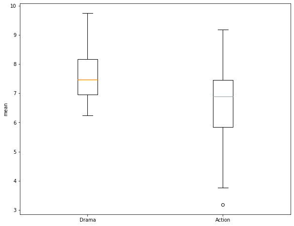
Before performing the test, I use matplotlib to create a grouped box plot to compare the central tendency and distribution of the two groups. Note that the interquartile ranges (IQR) overlap some and that there is a good bit of variability within the groups. So, it is not clear if there is actually a difference between the group means.
fig, ax = plt.subplots(1, 1)
ax.boxplot([mDa, mAa])
ax.set_xticklabels(["Drama", "Action"])
ax.set_ylabel("mean")
plt.show()
I am now ready to perform the Two-Sample T-Test. This function requires the two numpy arrays storing the values for each group. I also set the equal_var argument to False so that a Welch's T-Test will be performed and equal variance between groups is not assumed.
I obtain a T-Value of 3.11 and a p-value of 0.0031. Using an alpha of 0.05, we would reject the null hypothesis that the means between the two groups are not different because the obtained p-value is smaller than 0.05. We would favor the alternative hypothesis that the means between the two groups are different.
st.ttest_ind(mDa, mAa, equal_var=False)
Ttest_indResult(statistic=3.1125302908342998, pvalue=0.003104205237585028)
One-Way ANOVA
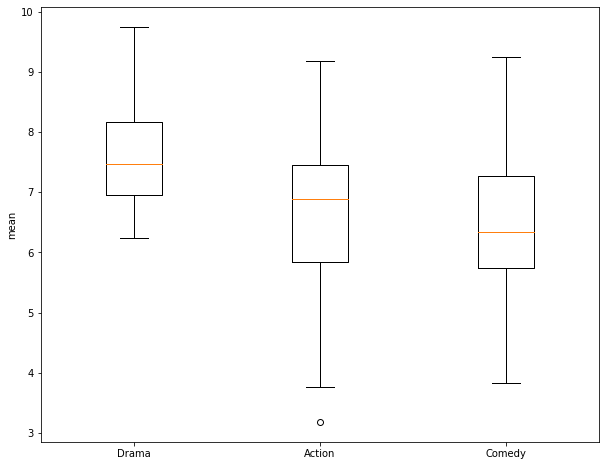
In this section, I demonstrate the use of a One-Way ANOVA to assess for differences in the means of multiple groups. First, I extract out 30 samples from the Comedy genera and generate a numpy array of the ratings. Next, I create a box plot to compare the three groups: Action, Drama, and Comedy. Again, it is not clear if the means are different between pairs of the three groups.
mC = movies_df.query('Genre=="Comedy"')
np.random.seed(42)
mC = mC.sample(30)
mCa = mC[mC.columns[3]].to_numpy()
fig, ax = plt.subplots(1, 1)
ax.boxplot([mDa, mAa, mCa])
ax.set_xticklabels(["Drama", "Action", "Comedy"])
ax.set_ylabel("mean")
plt.show()
To perform the ANOVA test, the numpy arrays of the ratings for each of the three groups are provided to the f_oneway() function. For my samples, I obtain an F-Value of 7.93 and a p-value of 0.000685. This suggest rejection of the null hypothesis in favor of the alternative hypothesis that at least two of the groups have different means. However, ANOVA does not tell us which of the groups are estimated to have different means. So, I next perform a Tukey-HSD test as a pairwise comparison. This is accomplished using the pairwise_tukeyhsd() function from the statsmodels library. This function expects the data to be provided differently than the T-Test and ANOVA already performed. Specifically, it requires all of the values to be provided as a single array and all of the group names to be provided as a separate array. To accomplish this, I copy one array and append all of the other rating values into it. I then create arrays containing 30 replicates of the group names then append them to a single array.
The Tukey-HSD test suggests that the Drama and Comedies and Drama and Action genres have different mean ratings while the Action and Comedies do not. Note that a p-value of less than 0.05 and a confidence interval that does not include zero suggests to reject the null hypothesis.
anovaF, anovaP = st.f_oneway(mAa, mDa, mCa)
print(anovaF)
print(anovaP)
7.932685401667139
0.0006845063246528356
forTHSD = np.copy(mAa)
forTHSD = np.append(forTHSD, mDa)
forTHSD = np.append(forTHSD, mCa)
grpsA = np.repeat(["Action"], 30)
grpsD = np.repeat(["Drama"], 30)
grpsC = np.repeat(["Comedy"], 30)
grps = np.copy(grpsA)
grps = np.append(grps, grpsD)
grps = np.append(grps, grpsC)
print(forTHSD)
print(grps)
[6.02 6.76 8.89 7.21 5.35 3.77 7.33 7.55 8.72 4.82 4.46 8.9  5.03 7.48
 6.73 6.73 5.86 9.18 7.23 3.18 6.76 7.01 6.03 7.84 7.06 7.34 5.84 4.51
 8.13 7.33 7.1  7.95 8.45 7.86 6.59 7.94 6.87 7.03 7.44 6.93 9.47 6.84
 8.52 7.95 6.43 6.55 9.35 7.67 7.73 8.23 7.23 7.1  7.48 6.68 6.24 9.75
 7.34 8.43 9.39 7.21 8.55 6.78 6.15 6.87 5.73 5.34 4.87 5.96 4.66 6.77
 7.47 6.09 5.48 3.83 4.01 6.74 6.03 7.87 7.35 5.23 8.21 7.57 6.38 5.8
 6.28 5.83 6.54 8.23 9.25 7.  ]
['Action' 'Action' 'Action' 'Action' 'Action' 'Action' 'Action' 'Action'
 'Action' 'Action' 'Action' 'Action' 'Action' 'Action' 'Action' 'Action'
 'Action' 'Action' 'Action' 'Action' 'Action' 'Action' 'Action' 'Action'
 'Action' 'Action' 'Action' 'Action' 'Action' 'Action' 'Drama' 'Drama'
 'Drama' 'Drama' 'Drama' 'Drama' 'Drama' 'Drama' 'Drama' 'Drama' 'Drama'
 'Drama' 'Drama' 'Drama' 'Drama' 'Drama' 'Drama' 'Drama' 'Drama' 'Drama'
 'Drama' 'Drama' 'Drama' 'Drama' 'Drama' 'Drama' 'Drama' 'Drama' 'Drama'
 'Drama' 'Comedy' 'Comedy' 'Comedy' 'Comedy' 'Comedy' 'Comedy' 'Comedy'
 'Comedy' 'Comedy' 'Comedy' 'Comedy' 'Comedy' 'Comedy' 'Comedy' 'Comedy'
 'Comedy' 'Comedy' 'Comedy' 'Comedy' 'Comedy' 'Comedy' 'Comedy' 'Comedy'
 'Comedy' 'Comedy' 'Comedy' 'Comedy' 'Comedy' 'Comedy' 'Comedy']
tukRes = pairwise_tukeyhsd(forTHSD, grps)
print(tukRes)
Multiple Comparison of Means - Tukey HSD, FWER=0.05
===================================================
group1 group2 meandiff p-adj   lower  upper  reject
---------------------------------------------------
Action Comedy   -0.206  0.788 -0.9943 0.5823  False
Action  Drama   1.0233 0.0074   0.235 1.8116   True
Comedy  Drama   1.2293  0.001   0.441 2.0176   True
---------------------------------------------------
Correlations
In this section, I assess the correlation between the movie rating and release year. This assessment could be used to determine whether there is a pattern in my brother's ratings over time. For example, does my brother tend to rate newer or older movies higher? I will specifically explore correlation for all of the dramas in the dataset. So, I extract out all of the dramas then write the ratings and release year to separate numpy arrays.
The Pearson Correlation Coefficient can be obtained using the pearsonr() function from stats. This metric assesses for a linear correlation between two continuous variables. Here, I obtain a correlation of -0.028, which has an associated p-value of 0.685. This suggests that there is not a strong linear relationship between the rating and release year. Or, my brother's ratings for dramas do not seem to vary based on release year.
The Spearman Correlation Coefficient can be obtained using the spearmanr() function, which assesses for a monotonic relationship using ranks. Here, I obtain a correlation of 0.006 with an associated p-value of 0.914. This again suggests that there is not a strong monotonic relationship between the movie rating and release year.
mD = movies_df.query('Genre=="Drama"')
mDr = mD[mD.columns[3]].to_numpy()
mDy = mD[mD.columns[2]].to_numpy()
print(st.pearsonr(mDr, mDy))
(-0.022701968234130208, 0.6853270459162113)
print(st.spearmanr(mDr, mDy))
SpearmanrResult(correlation=0.006073936628682969, pvalue=0.9136784076967588)
Linear Regression
In this last section, I will demonstrate implementing linear regression using scikit-learn. First, I will estimate average mean county temperature using the mean county elevation. I will then undertake multiple linear regression by predicting the mean county temperature using elevation, percent forest cover, and mean county total annual precipitation.
First, I read in the "high_plains_data.csv" file. These data represent environmental and climate data for counties in the high plains states. The climate data were derived from PRISM, and the land cover data were derived from the National Land Cover Database (NLCD).
hp = pd.read_csv("D:/mydata/high_plains_data.csv", sep=",", header=0, encoding="ISO-8859-1")
hp.columns =[column.replace(" ", "_") for column in hp.columns]
print(hp.head(10))
   GEOID10    ID             NAME_1 STATE_NAME ST_ABBREV         AREA  \
0     8053  8053    Hinsdale County   Colorado        CO  1123.212157
1     8061  8061       Kiowa County   Colorado        CO  1785.889183
2     8063  8063  Kit Carson County   Colorado        CO  2161.740894
3     8071  8071  Las Animas County   Colorado        CO  4775.291392
4     8073  8073     Lincoln County   Colorado        CO  2586.326731
5     8075  8075       Logan County   Colorado        CO  1845.045782
6     8079  8079     Mineral County   Colorado        CO   877.691373
7     8085  8085    Montrose County   Colorado        CO  2242.693513
8     8087  8087      Morgan County   Colorado        CO  1293.760087
9     8089  8089       Otero County   Colorado        CO  1269.475894

   TOTPOP10  POPDENS10  MALES10  FEMALES10  ...  TOTHH00  FAMHH00  TOTHU00  \
0       843        0.8      443        400  ...      359      247     1304
1      1398        0.8      687        711  ...      665      452      817
2      8270        3.8     4638       3632  ...     2990     2081     3430
3     15507        3.2     7948       7559  ...     6173     4095     7629
4      5467        2.1     3163       2304  ...     2058     1389     2406
5     22709       12.4    12924       9785  ...     7551     5064     8424
6       712        0.8      362        350  ...      377      251     1119
7     41276       18.4    20310      20966  ...    13043     9311    14202
8     28159       22.0    13898      14261  ...     9539     6969    10410
9     18831       14.9     9221       9610  ...     7920     5473     8813

   OWNER00  RENTER00    per_for         elev       temp      precip   precip2
0      233       126  34.962704  3334.739362   1.410638  800.246066  8.002461
1      474       191   0.002120  1269.637288  11.159492  384.201797  3.842018
2     2151       839   0.021467  1348.005495  10.179698  435.414037  4.354140
3     4360      1813  11.687193  1834.354115  10.439925  424.757731  4.247577
4     1421       637   0.043238  1564.500000   9.573578  376.228555  3.762286
5     5277      2274   0.124509  1278.251592   9.749204  425.278696  4.252787
6      279        98  38.846741  3212.506757   1.830405  856.293446  8.562934
7     9773      3270  33.571025  2122.834667   8.327253  447.202160  4.472022
8     6525      3014   0.112152  1372.481651   9.731422  369.794908  3.697949
9     5471      2449   0.024750  1355.050926  11.780972  338.015001  3.380150

[10 rows x 157 columns]
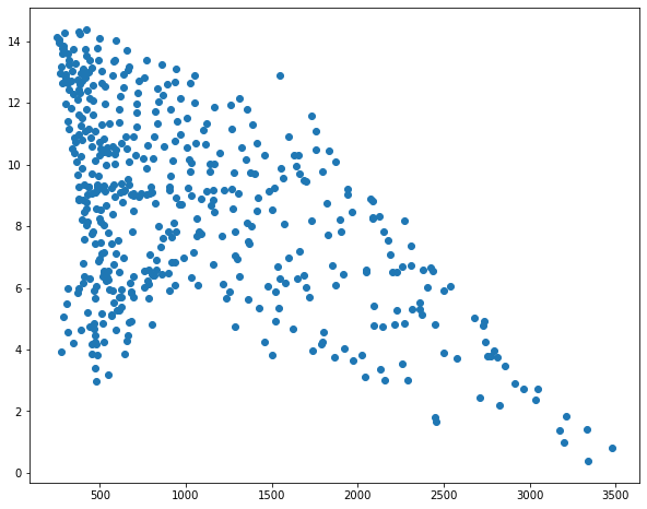
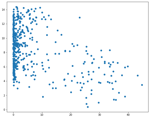
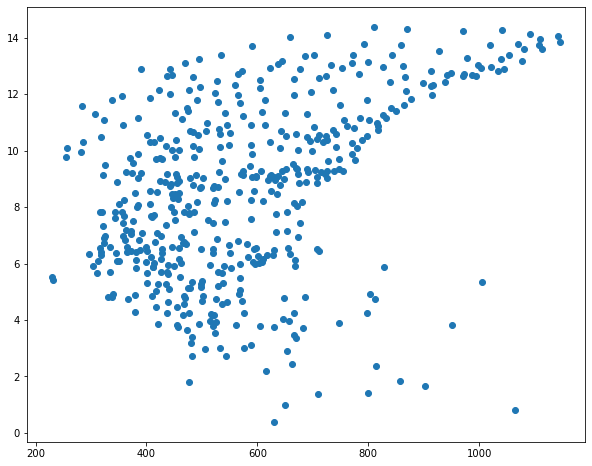
I then use matplotlib to create scatter plots to visualize the relationship between temperature and the three predictor variables. Generally, there seems to be a stronger correlation between temperature and elevation in comparison to temperature and the other two variables.
sp1 = plt.scatter(hp.elev, hp.temp)
plt.show(sp1)
sp1 = plt.scatter(hp.per_for, hp.temp)
plt.show(sp1)
sp1 = plt.scatter(hp.precip, hp.temp)
plt.show(sp1)
I subset out the temperature data and predictor variables into separate data frames. I then split the data into separate training and testing sets using the train_test_split() function from scikit-learn. This function requires that both the predictor variables and dependent variable be provided. You must also specify the proportion of the data to maintain for testing. A random state can be specified to allow for reproducibility.
yvar = hp[["temp"]]
xvars= hp[["elev", "per_for", "precip"]]
X_train, X_test, y_train, y_test = train_test_split(xvars,
yvar, test_size=0.33, random_state=42)
X_trainElev = X_train[["elev"]]
X_testElev = X_test[["elev"]]
print(yvar.head())
print(xvars.head())
        temp
0   1.410638
1  11.159492
2  10.179698
3  10.439925
4   9.573578
          elev    per_for      precip
0  3334.739362  34.962704  800.246066
1  1269.637288   0.002120  384.201797
2  1348.005495   0.021467  435.414037
3  1834.354115  11.687193  424.757731
4  1564.500000   0.043238  376.228555
I next initiate a model and fit using the training data and only the elevation predictor variable. Once the model is fit, I can obtain the intercept and coefficient. So, the resulting formula is:
Temperature = 10.8 - 0.00219*Elevation.
I then predict to the withheld test data and use the results to calculate the root mean square error or RMSE. The model resultd in an RMSE of 2.66, which suggests that the predicted temperature is off by 2.66 degrees Celsius on average for the withheld counties.
lmMod = LinearRegression()
lmMod.fit(X_trainElev, y_train)
LinearRegression()
print(f"intercept: {lmMod.intercept_}")

print(f"coefficients: {lmMod.coef_}")
intercept: [10.80000493]
coefficients: [[-0.00219406]]
preds = lmMod.predict(X_testElev)
mean_squared_error(y_test, preds, squared=False)
2.658858018975682
I now fit a new model using all three predictor variables. This results in a fitted y-intercept and three coefficients, one for each predictor variable. The RMSE actually increases to 2.89, suggesting that including of the precipitation and percent forest cover variables did not improve the model performance in comparison to just using the mean county elevation.
lmMod = LinearRegression()
lmMod.fit(X_train, y_train)
LinearRegression()
print(f"intercept: {lmMod.intercept_}")

print(f"coefficients: {lmMod.coef_}")
intercept: [2.58132095]
coefficients: [[ 0.00113803 -0.20148305  0.0105595 ]]
preds = lmMod.predict(X_test)
mean_squared_error(y_test, preds, squared=False)
2.887478419012105
Concluding Remarks
This short module provided a brief introduction to performing statistical tests and linear regression in Python. If you need to perform different tests, I think you will find that the syntax is very similar. The general workflow is to (1) read in the required data, (2) prepare the data so that it can be provided to the test of interest, (3) implement the test, and (4) interpret the results. It is important to note that most tests have assumptions that should be evaluated to make sure the results are not misleading. We will further explore predictive modeling using scikit-learn in the machine learning module.