Raster Analysis with terra

Objectives

Compare the terra and raster packages for working with and analyzing raster data
Convert scripts that used raster to incorporate terra
Use terra for raster analysis
Use the terra documentation

Overview

The raster package has been a central tool for working with geospatial data in R. However, recently the originators of raster have released the terra package, which has been designed to replace raster. The raster package can be slow and can result in memory issues if large raster data sets are used. terra works to alleviate some of these issues. First, it is very fast since it makes use of C++ code. It also supports working with larger data sets as it is not required to read entire raster grids into memory.

Since terra is fairly new, I have decided to maintain the material relating to the raster package for the time being. However, it is important to introduce terra. Eventually, I plan to remove our raster package content and maintain only the terra content.

In order to investigate terra, we will re-execute some of the processes explored in prior modules using terra as opposed to raster with a focus on highlighting differences in the syntax and implementation.

Here are some helpful links for learning terra:

The terra package introduces the following new classes:

SpatRaster: for raster data and limits memory usage in comparison to the raster package data models
SpatVector: represent vector-based point, line, or polygon features and their associated attributes.
SpatExtent: for spatial extent information derived from a SpatRaster or SpatVector or manually defined.

Although we will not explore it directly here, the stars package offers additional functionality to efficient work with spatial data including spatiotemporal arrays, raster data cubes, and vector data cubes. The documentation for this package is available here.

The link at the bottom of the page provides the example data and R Markdown file used to generate this module.

Reading in Data

First, I will read in the required packages. Note that terra relies on C++, so you will need to have the Rcpp package installed, which allows for R and C++ integration.

library(terra)
library(tmap)
library(rgdal)
library(tmaptools)
library(sf)
library(dplyr)

Instead of generating or reading in raster grids using raster(), brick(), or stack(), all raster grids, regardless of the number of bands, are created or read in using the rast() function. In the following code block, I first created a raster grid by defining the number of rows, columns, min/max coordinates, and spatial reference information. Next, I read in single-band data followed by multi-band data. In all cases, the rast() function is used and objects of the SpatRaster class are created. The tmap package can still be used to display the resulting raster grids. The terra package also provides plot() and plotRGB() functions for visualizing data.

#Build raster data from scratch
basic_raster <- rast(ncols = 10, nrows = 10, xmin = 500000, xmax = 500100, ymin = 4200000, ymax = 4200100, crs="+init=EPSG:26917")
vals <- sample(c(0:255), 100, replace=TRUE)

values(basic_raster) <- vals

tm_shape(basic_raster)+
  tm_raster()+
  tm_layout(legend.outside = TRUE)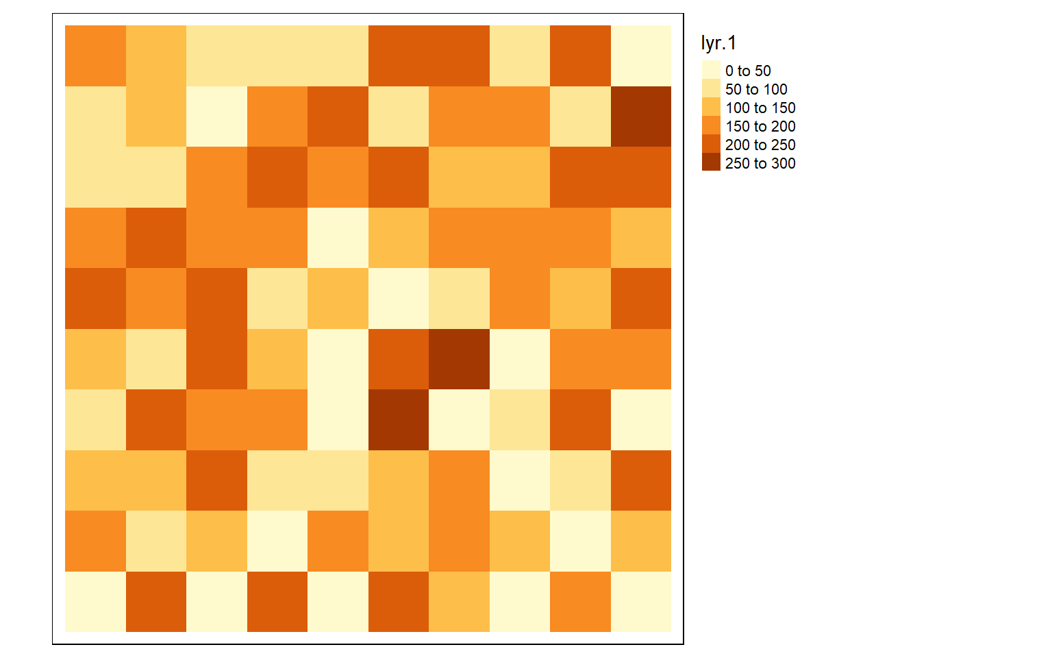

#Read in single-band data
dem <- rast("terra/from_spatial_data/dem_example.tif")
lc <- rast("terra/from_spatial_data/lc_example.tif")

tm_shape(lc)+
  tm_raster(style= "cat",
            labels = c("Open Water", "Developed Open", "Developed Low Int.", "Developed Med. Int.", "Developed High Int.", "Barren", "Deciduous Forest", "Evergreen Forest", "Mixed Forest", "Pasture/Hay", "Cultivated Crop", "Woody Wetland", "Emergent Wetland"),
            palette = c("deepskyblue", "brown1", "brown2", "brown3", "brown4", "darkgrey", "darkolivegreen", "darkolivegreen1", "darkseagreen1", "goldenrod3", "darkorange", "darkorchid1", "darkorchid4"),
            title="Land Cover")+
  tm_layout(legend.outside = TRUE)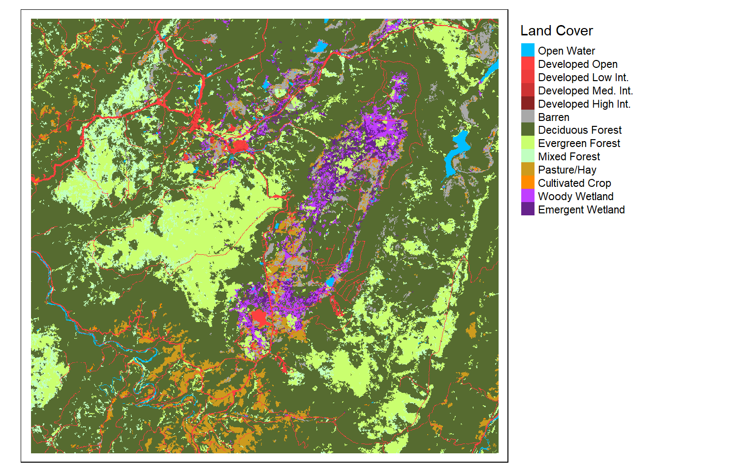

tm_shape(dem)+
  tm_raster(style= "cont", palette=get_brewer_pal("-Greys", plot=FALSE))+
  tm_layout(legend.outside = TRUE)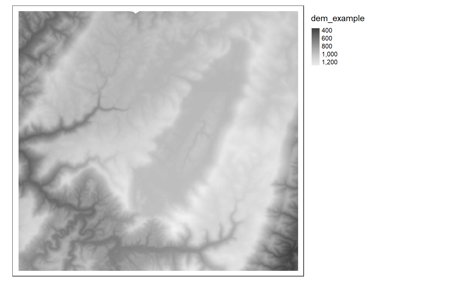

#Read in multiband data
s1 <- rast("terra/from_spatial_data/sentinel_vancouver.tif")

plotRGB(s1, r=4, g=3, b=2, stretch="lin")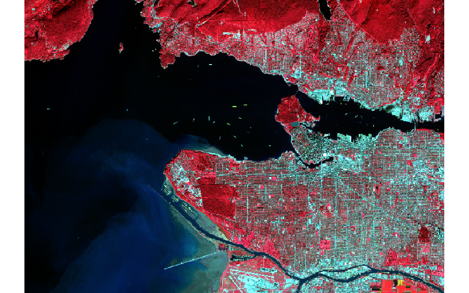

plotRGB(s1, r=5, g=4, b=2, stretch="lin")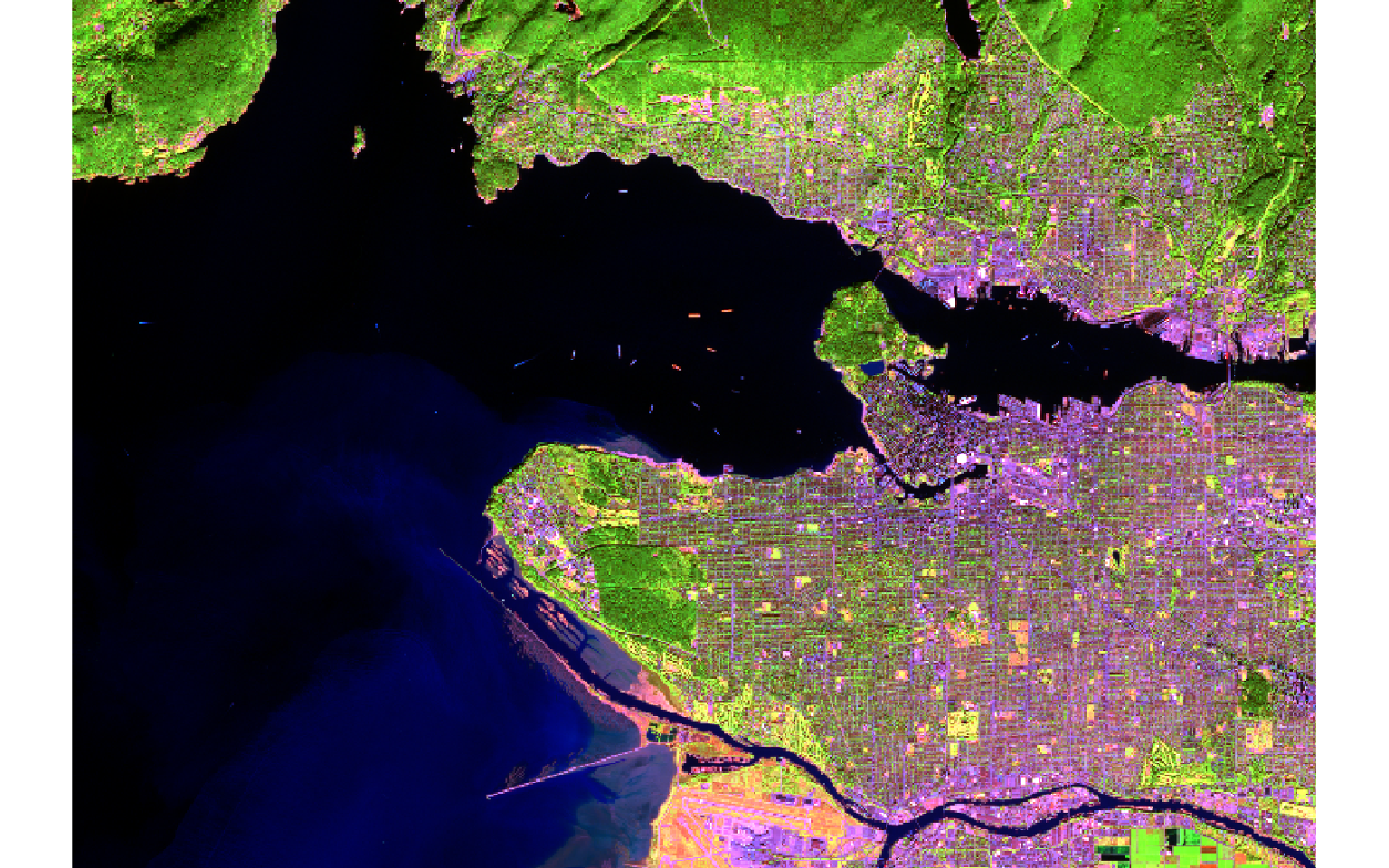

Basic Data Manipulation

The following examples show how to crop, merge, mask, aggregate, and reclassify raster data using terra. Terra also contains data models for vector data. Vector data can be read in using the vect() function, which generates an object of the SpatVector class. In the masking example, vector-based watershed boundaries are used to mask the digital elevation data. Currently, SpatVector objects cannot be used in tmap. So, I also read the vector data with sf to generate a data frame.

Raster reclassification is performed with the classify() function.

# Read in example data
elev <- rast("terra/from_raster_analysis/elevation1.tif")
slp <- rast("terra/from_raster_analysis/slope1.tif")
lc <- rast("terra/from_raster_analysis/lc_example.tif")

# Crop out extents
tm_shape(elev)+
  tm_raster(style= "cont")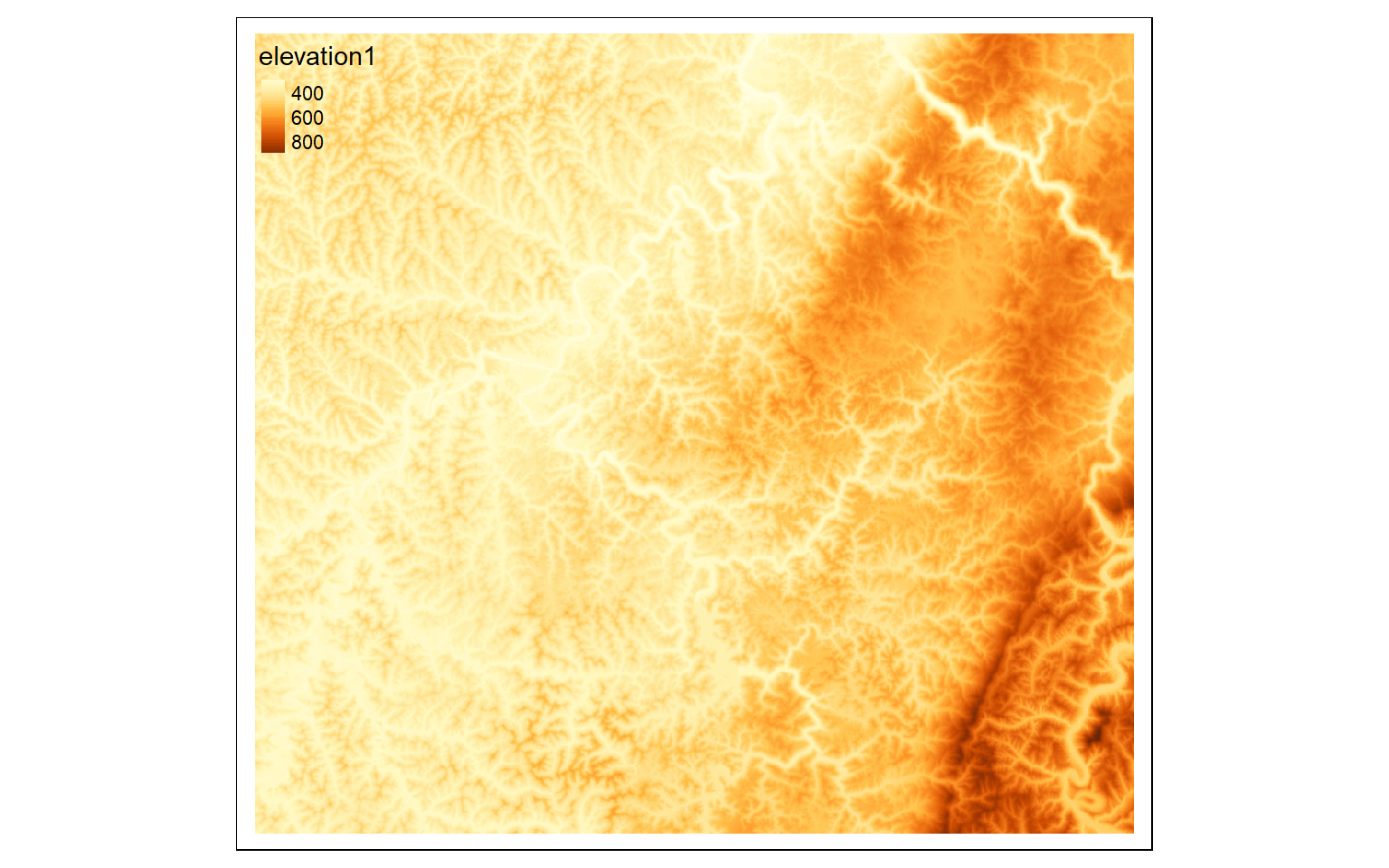

crop_extent <- ext(580000, 620000, 4350000, 4370000)
elev_crop <- crop(elev, crop_extent)

tm_shape(elev_crop)+
  tm_raster(style= "cont")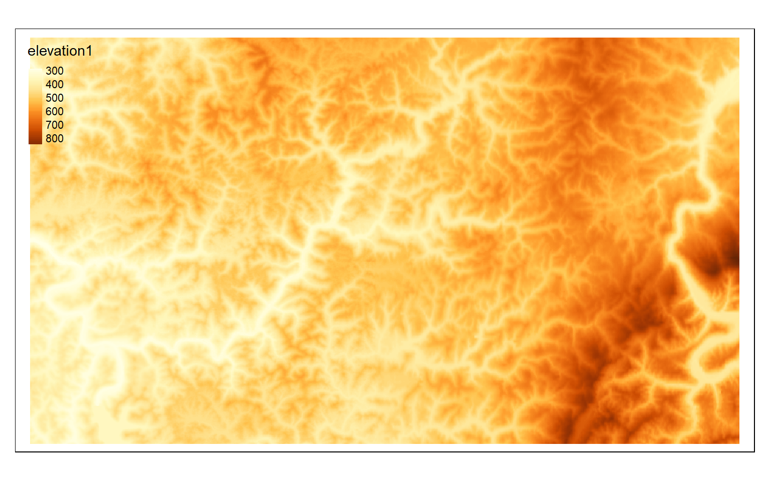

elev_crop2 <- crop(elev, ext(570000,600000, 432000,4360000))

#Merge cropped extents
elev_merge <- terra::merge(elev_crop, elev_crop2)

tm_shape(elev_merge)+
  tm_raster(style= "cont")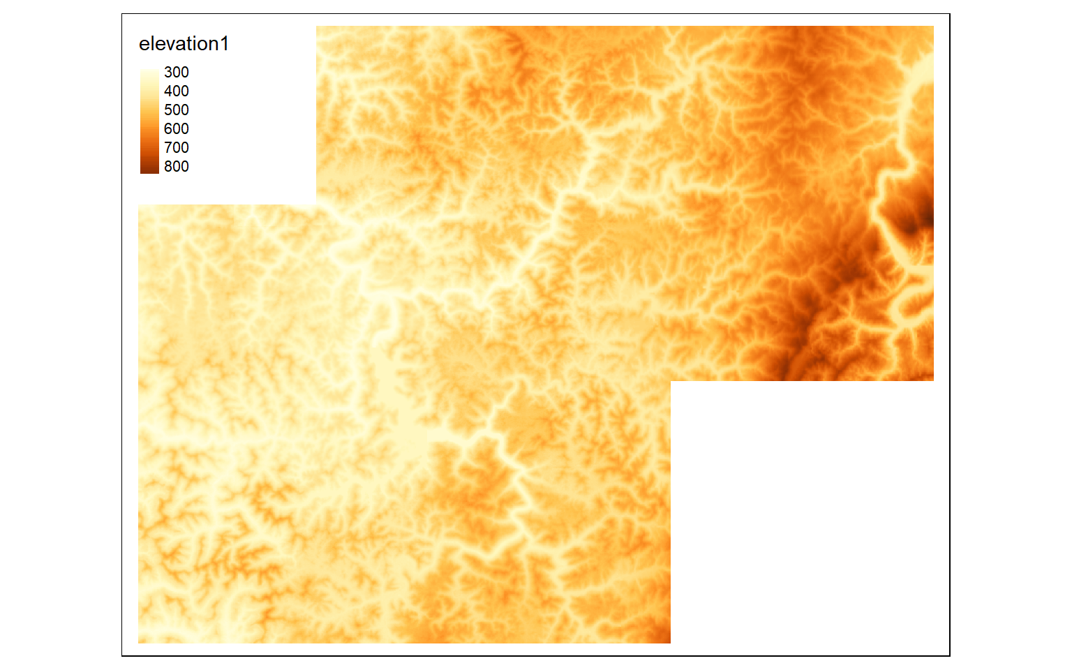

ws <- st_read("terra/from_raster_analysis/watersheds.shp")
Reading layer `watersheds' from data source 
  `C:\Maxwell_Data\Dropbox\Teaching_WVU\web_template\spatial_analytics_book\ossa\terra\from_raster_analysis\watersheds.shp' 
  using driver `ESRI Shapefile'
Simple feature collection with 11 features and 15 fields
Geometry type: POLYGON
Dimension:     XY
Bounding box:  xmin: 554473.9 ymin: 4337973 xmax: 610447.8 ymax: 4389046
Projected CRS: WGS 84 / UTM zone 17N
ws2 <- vect("terra/from_raster_analysis/watersheds.shp")

elev_mask <- mask(elev, ws2)

tm_shape(elev_mask)+
  tm_raster(style= "cont")+
  tm_shape(ws)+
  tm_borders(col="black")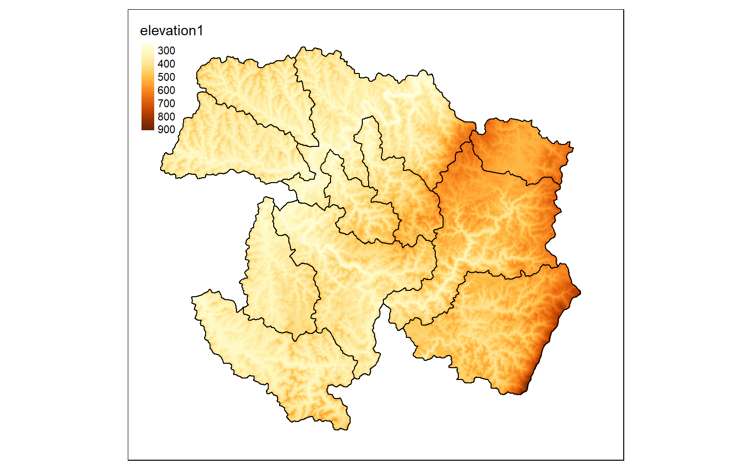

#Aggregate pixels
elev_agg <- aggregate(elev, fact=5, fun=mean)

m <- c(0, 300, 1,  300, 500, 2,  500,
       800,  3, 800, 10000, 4)
m <- matrix(m, ncol=3, byrow = TRUE)

dem_re <- classify(elev, m, right=TRUE)

tm_shape(dem_re)+
  tm_raster(style= "cat")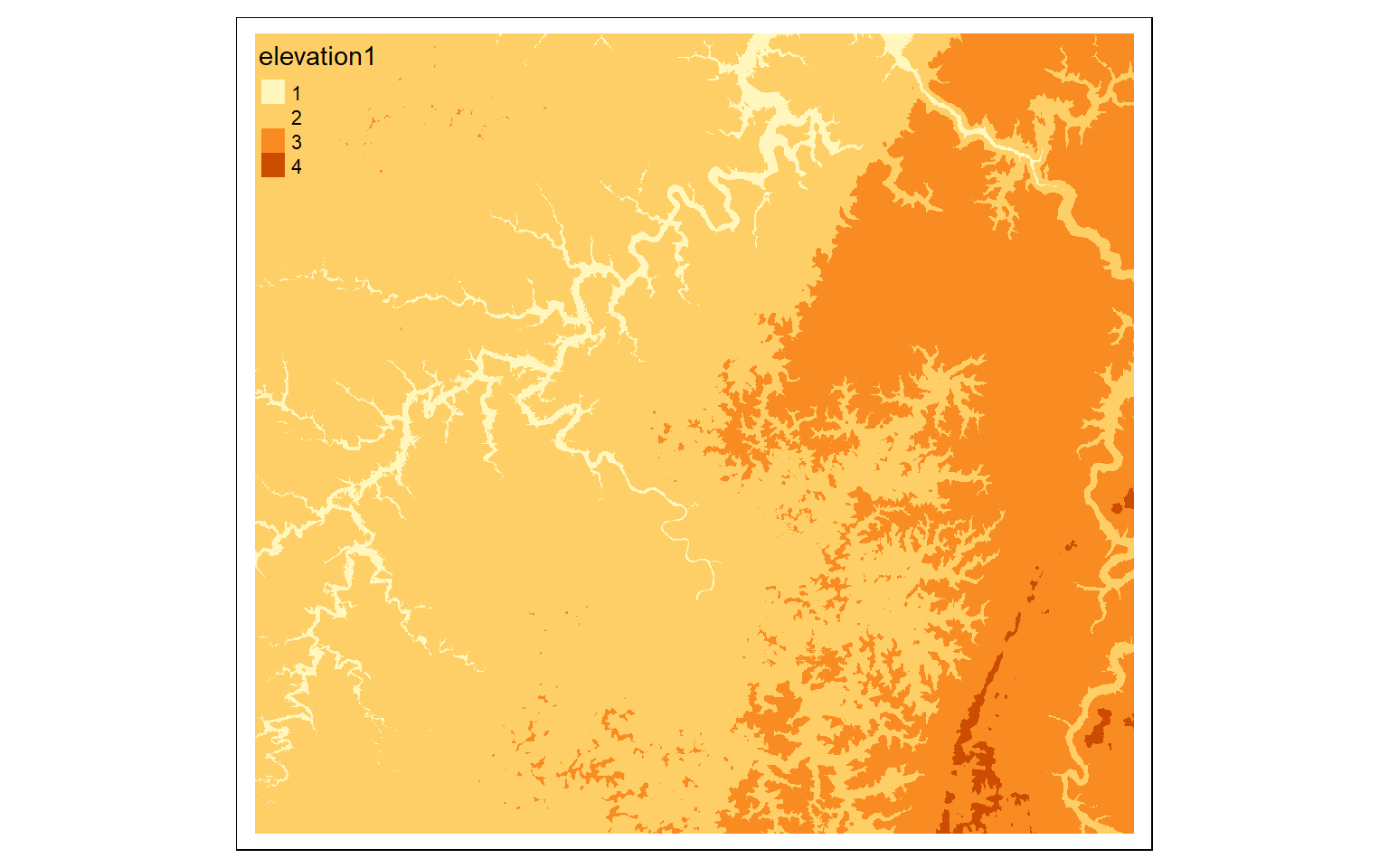

#Reclassify data
m2 <- c(10, 40, 0, 40, 50, 1, 50, 100, 0)
m2 <- matrix(m2, ncol=3, byrow = TRUE)

lc_re <- classify(lc, m2, right=TRUE)

tm_shape(lc_re)+
  tm_raster(style= "cat", labels = c("Not Forest", "Forest"), palette = c("gray", "darkolivegreen"))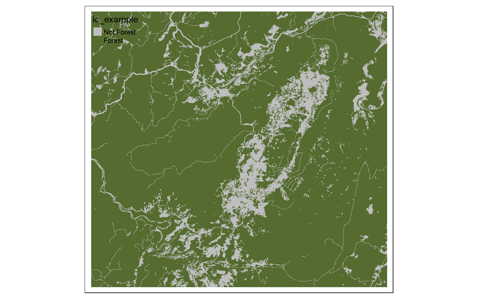

Raster Math

Raster math and logical operations are identical between raster and terra. So, once data are read in, you can use the same syntax as you would with raster to obtain binary grids or work with the raster values.

elev_ft <- elev*3.28084

tm_shape(elev_ft)+
  tm_raster(style= "cont")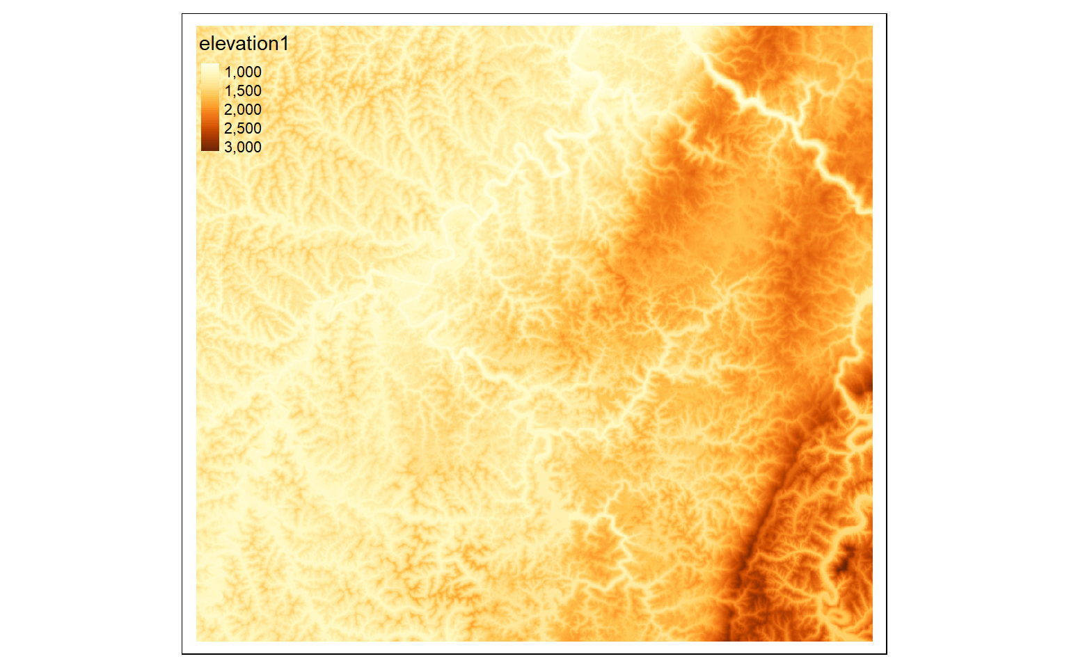

elev_600 <- elev > 600

tm_shape(elev_600)+
  tm_raster(style= "cat", labels = c("No", "Yes"), palette = c("gray", "darkred"))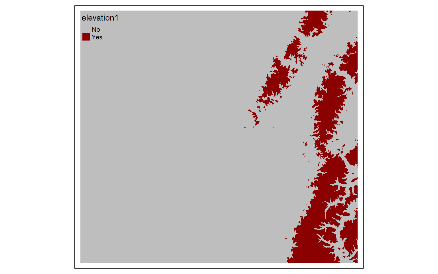

invert <- elev_600 == 0

tm_shape(invert)+
  tm_raster(style= "cat", labels = c("No", "Yes"), palette = c("gray", "darkred"))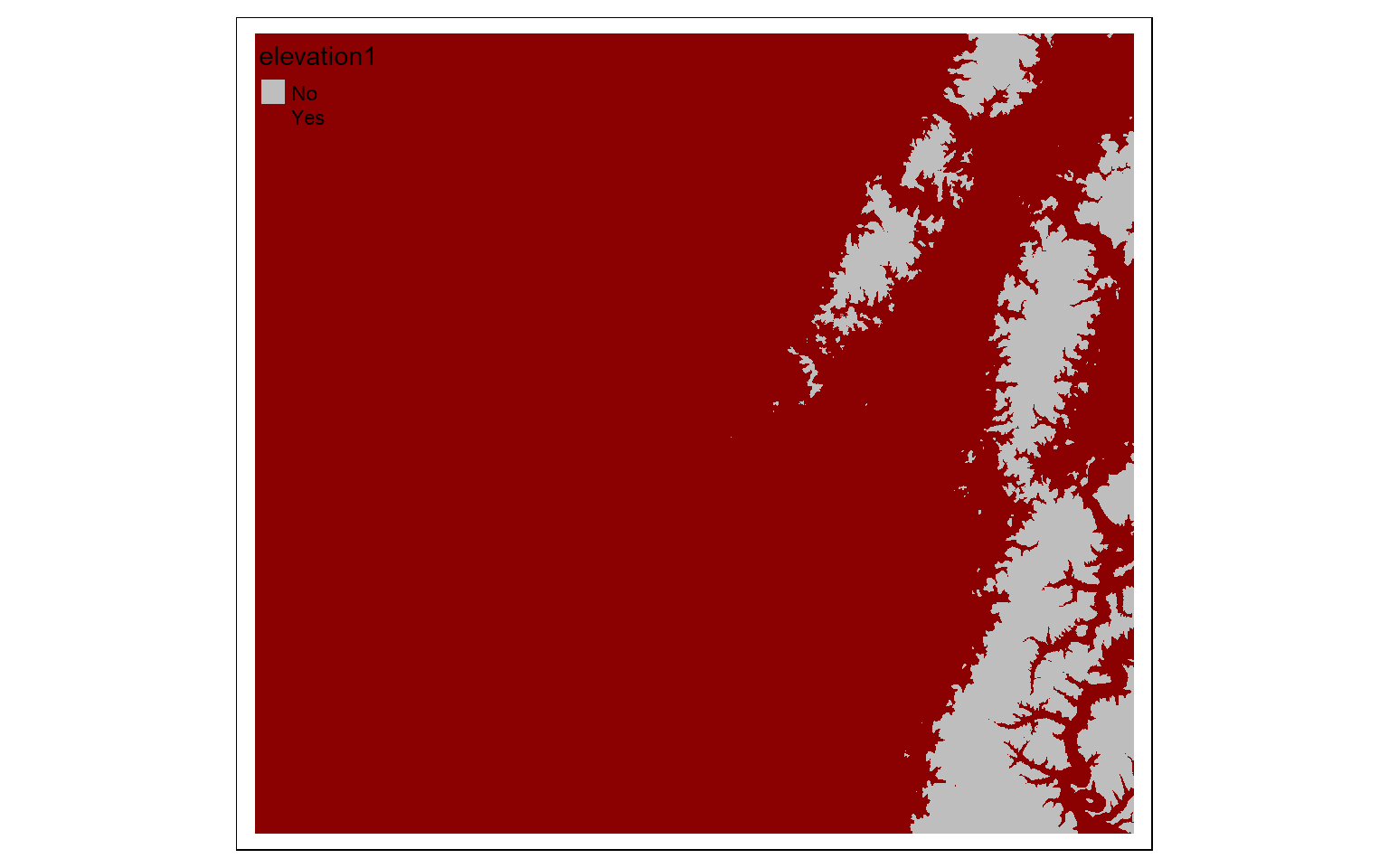

Summarize Raster Data

The extract() function can be used to extract raster values at point locations or obtain summary statistics within polygon or areal features. For areal features, you must provide a desired summary metric. Results are stored as SpatVector objects. In my examples, in order to obtain just a data frame with no geometric information, I use as.data.frame() and set the geom argument to NULL. I then merge the results with the input point or areal data read in using sf. This allows for the data to be plotted using tmap.

Based on my own experimentation, I have found extraction operations to be much faster with terra in comparison to raster.

pnts <- st_read("terra/from_raster_analysis/example_points.shp")
Reading layer `example_points' from data source 
  `C:\Maxwell_Data\Dropbox\Teaching_WVU\web_template\spatial_analytics_book\ossa\terra\from_raster_analysis\example_points.shp' 
  using driver `ESRI Shapefile'
Simple feature collection with 47 features and 1 field
Geometry type: POINT
Dimension:     XY
Bounding box:  xmin: 556505.6 ymin: 4341385 xmax: 608028.9 ymax: 4388863
Projected CRS: WGS 84 / UTM zone 17N
pnts2 <- vect("terra/from_raster_analysis/example_points.shp")

pnts_elev <- terra::extract(elev, pnts2, fun=mean)
pnts_elev2 <- as.data.frame(pnts_elev, geom=NULL)

pnts$elev <- as.numeric(pnts_elev2$elevation1)

tm_shape(elev)+
  tm_raster(style= "cont")+
  tm_shape(pnts)+
  tm_bubbles(size="elev")+
  tm_layout(legend.outside=TRUE)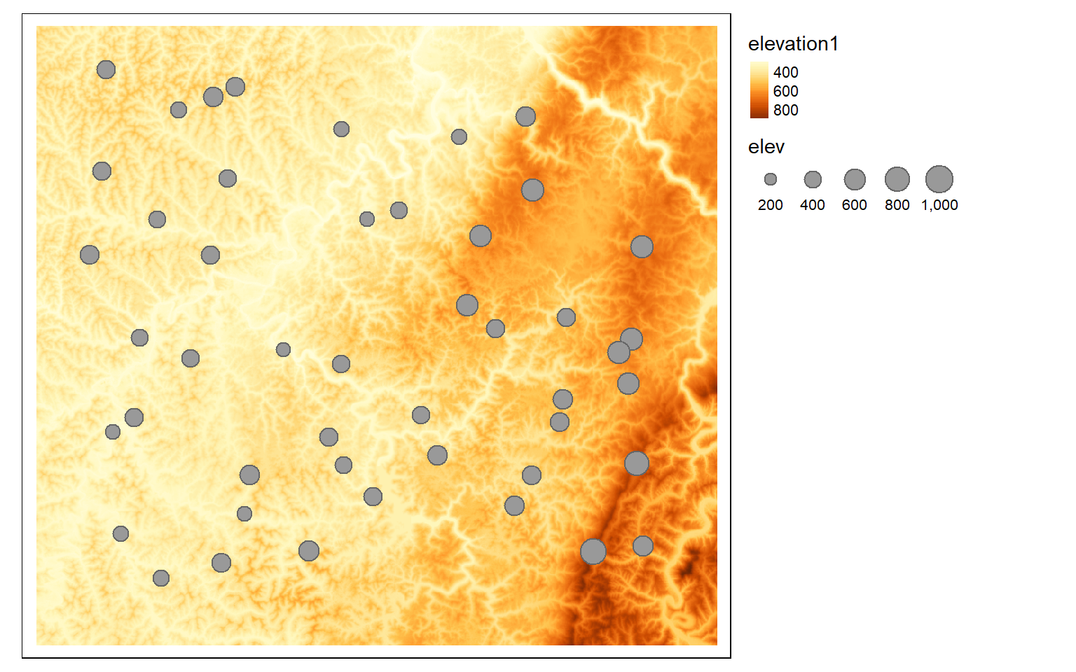

ws_mn_elev <- terra::extract(elev, ws2, fun=mean)
ws_mn_elev2 <- as.data.frame(ws_mn_elev, geom=NULL)

ws$elev <- as.numeric(ws_mn_elev2$elevation1)

tm_shape(ws)+
  tm_polygons(col="elev")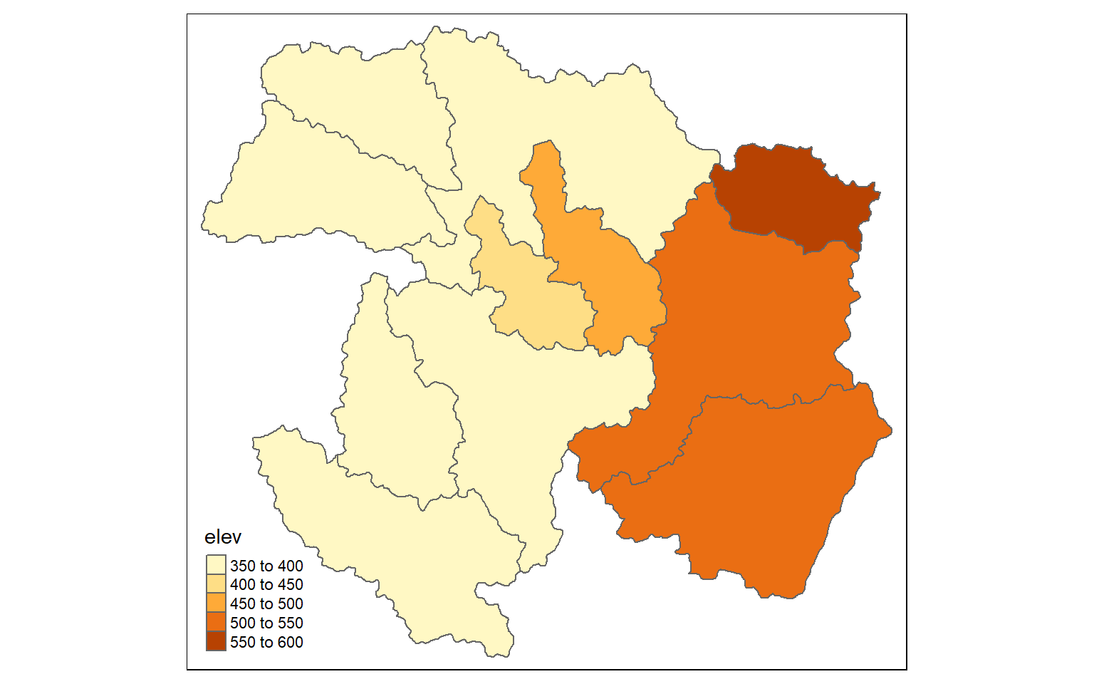

Distance Grids

Calculating Euclidean distance grids relative to points, lines, polygons, or raster cells is accomplished using the distance() function. There is no longer a need to convert line features to raster grids or points, as was the case with the raster package. If vector data are used as the source feature to which distance is calculated, they should be read in using vect(). Although distance calculations are simpler and faster in comparison to terra, my own experimentation suggests they are slower than ArcGIS Desktop, ArcGIS Pro, and QGIS. Similar to raster, terra is not capable of generating kernel density surfaces. Instead, you should use the sp.kde() function from the spatialEco() package.

air <- vect("terra/from_raster_analysis/airports.shp")
air2 <- st_read("terra/from_raster_analysis/airports.shp")
Reading layer `airports' from data source 
  `C:\Maxwell_Data\Dropbox\Teaching_WVU\web_template\spatial_analytics_book\ossa\terra\from_raster_analysis\airports.shp' 
  using driver `ESRI Shapefile'
Simple feature collection with 101 features and 9 fields
Geometry type: POINT
Dimension:     XY
Bounding box:  xmin: 363896.7 ymin: 4123139 xmax: 765733.2 ymax: 4497709
Projected CRS: WGS 84 / UTM zone 17N
dist <- distance(elev, air)

tm_shape(dist)+
  tm_raster(style= "cont")+
  tm_shape(air2)+
  tm_bubbles()+
  tm_layout(legend.outside=TRUE)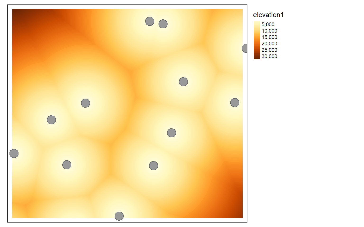

inter <- vect("terra/from_raster_analysis/interstates.shp")
inter2 <- st_read("terra/from_raster_analysis/interstates.shp")
Reading layer `interstates' from data source 
  `C:\Maxwell_Data\Dropbox\Teaching_WVU\web_template\spatial_analytics_book\ossa\terra\from_raster_analysis\interstates.shp' 
  using driver `ESRI Shapefile'
Simple feature collection with 47 features and 14 fields
Geometry type: LINESTRING
Dimension:     XY
Bounding box:  xmin: 360769.4 ymin: 4125421 xmax: 772219.7 ymax: 4438518
Projected CRS: WGS 84 / UTM zone 17N
dist2 <- distance(elev, inter)

tm_shape(dist2)+
  tm_raster(style= "cont")+
  tm_shape(inter2)+
  tm_lines(col="black")+
  tm_layout(legend.outside=TRUE)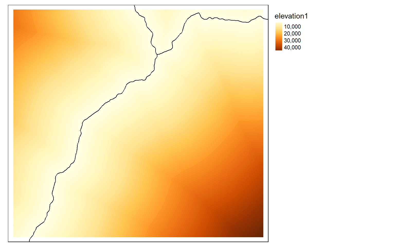

Conservative and Liberal Models

Generating conservative (i.e., binary) or liberal models using terra is the same as the process implemented using raster once all input grids are read in or created. The process of generating binary grids, rescaling grids, multiplying grids by weights, and adding scored grids together is the same. One difference is that the global() function must be used to obtain summary statistics used in the data rescaling, such as the minimum and maximum values in a grid. In the example, I obtain minimum and maximum values using global() and use as.vector() to return the single value as a vector object. I also make sure to ignore null values.

# Conservative Model

#Elevation > 500
#Slope < 15
#Airports < 3000
#Interstates < 5000

elev_binary <- elev > 500
ele_b <- tm_shape(elev_binary)+
  tm_raster(style="cat")+
  tm_layout(main.title="Elevation")

slp_binary <- slp < 15
slp_b <- tm_shape(slp_binary)+
  tm_raster(style="cat")+
  tm_layout(main.title="Slope")

air_binary <- dist < 7000
airport_b <- tm_shape(air_binary)+
  tm_raster(style="cat")+
  tm_layout(main.title="Airports")

inter_binary <- dist2 < 5000
interstate_b <- tm_shape(inter_binary)+
  tm_raster(style="cat")+
  tm_layout(main.title="Interstates")

tmap_arrange(ele_b, slp_b, airport_b, interstate_b)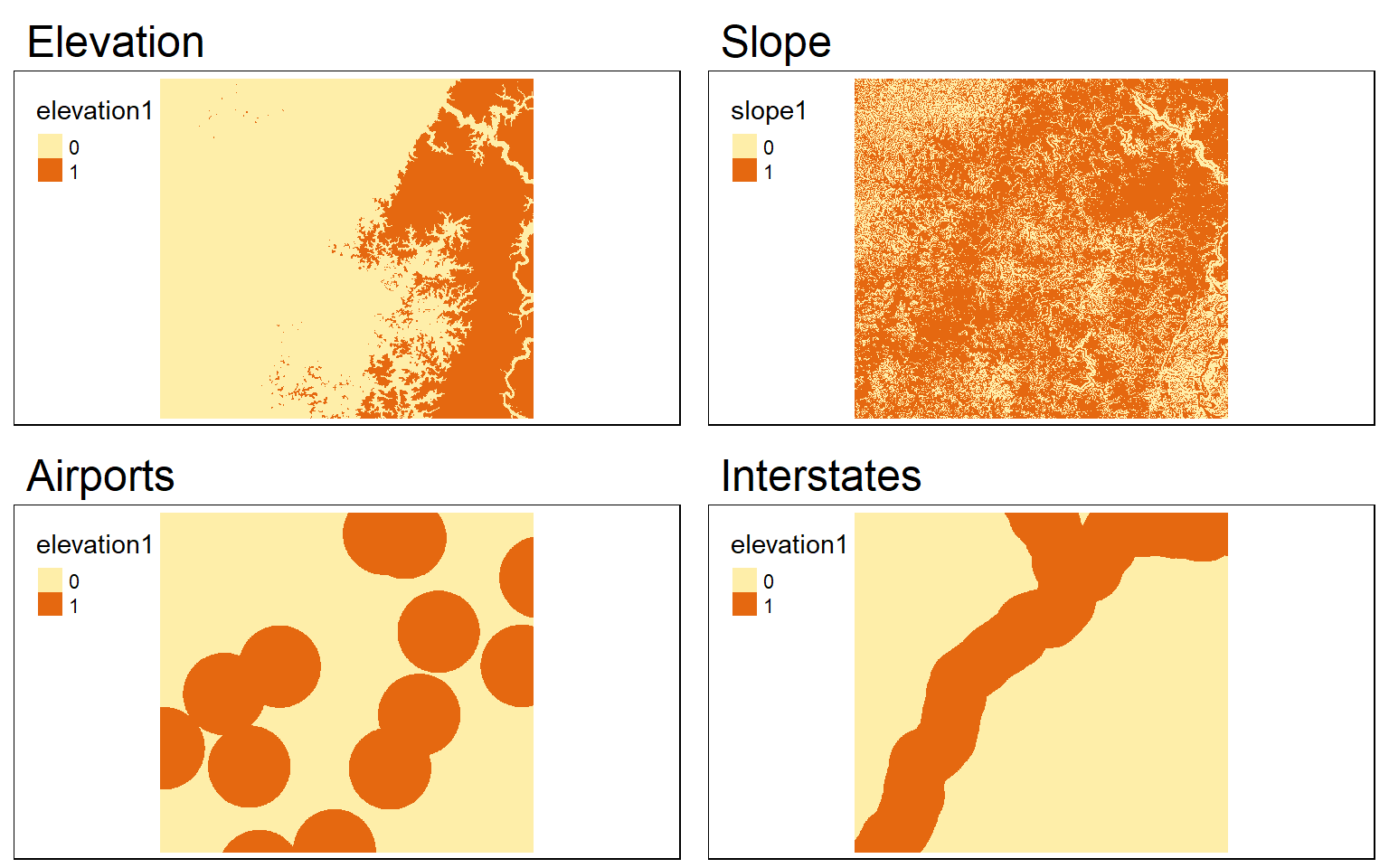

c_model <- elev_binary*slp_binary*air_binary*inter_binary

tm_shape(c_model)+
  tm_raster(style="cat")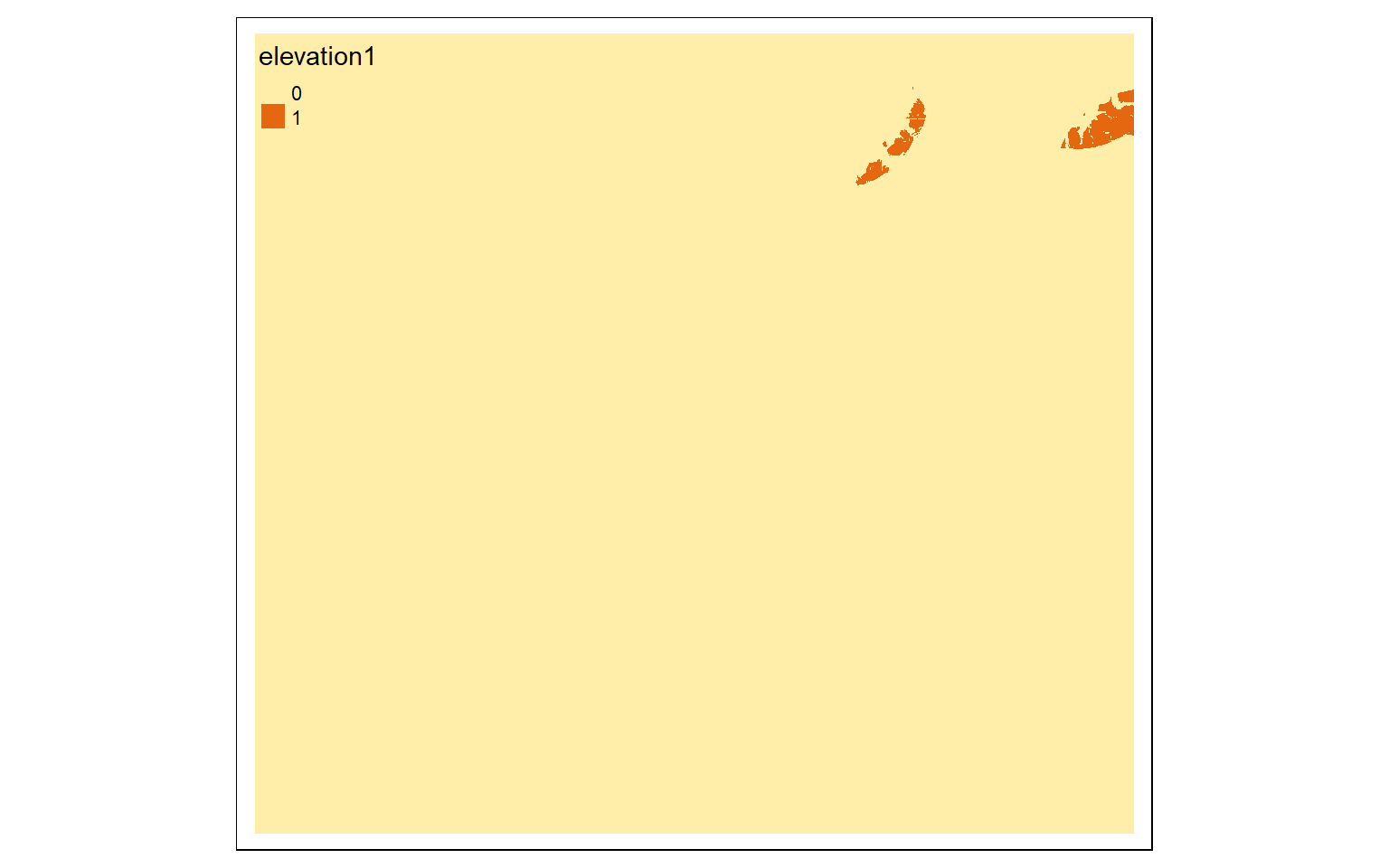

#Liberal Model
#High elevation is good
#Low slope is good
#Close to airports is good
#Close to interstates is good

elev_min <- as.vector(global(elev, fun=min, na.rm=TRUE)[1,1])
elev_max <- as.vector(global(elev, fun=max, na.rm=TRUE)[1,1])
elev_score <- ((elev - elev_min)/(elev_max - elev_min))
ele_s <- tm_shape(elev_score)+
  tm_raster(style="cont")+
  tm_layout(main.title="Elevation")

slp_min <- as.vector(global(slp, fun=min, na.rm=TRUE)[1,1])
slp_max <- as.vector(global(slp, fun=max, na.rm=TRUE)[1,1])
slp_score <- 1 - ((slp - slp_min)/(slp_max - slp_min))
slp_s <- tm_shape(slp_score)+
  tm_raster(style="cont")+
  tm_layout(main.title="Slope")

air_min <- as.vector(global(dist, fun=min, na.rm=TRUE)[1,1])
air_max <- as.vector(global(dist, fun=max, na.rm=TRUE)[1,1])
air_score <- 1 - ((dist - air_min)/(air_max - air_min))
airport_s <- tm_shape(air_score)+
  tm_raster(style="cont")+
  tm_layout(main.title="Airports")

inter_min <- as.vector(global(dist2, fun=min, na.rm=TRUE)[1,1])
inter_max <- as.vector(global(dist2, fun=max, na.rm=TRUE)[1,1])
inter_score <- 1- (dist2 - inter_min)/(inter_max - inter_min)
interstate_s <- tm_shape(inter_score)+
  tm_raster(style="cont")+
  tm_layout(main.title="Interstates")

tmap_arrange(ele_s, slp_s, airport_s, interstate_s)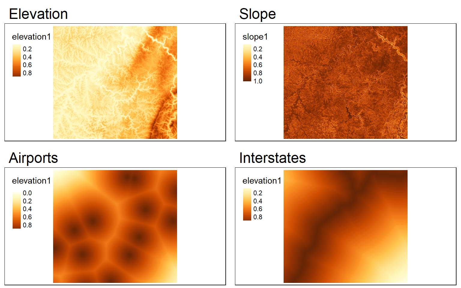

#Weight for elevation = 0.1
#Weight for slope =0.4
#Weight for Airport Distance = 0.2
#Weight for Interstate Distance =0.3

wo_model <- (elev_score*.1)+(slp_score*.4)+(air_score*.2)+(inter_score*.3)

tm_shape(wo_model)+
  tm_raster(style="cont")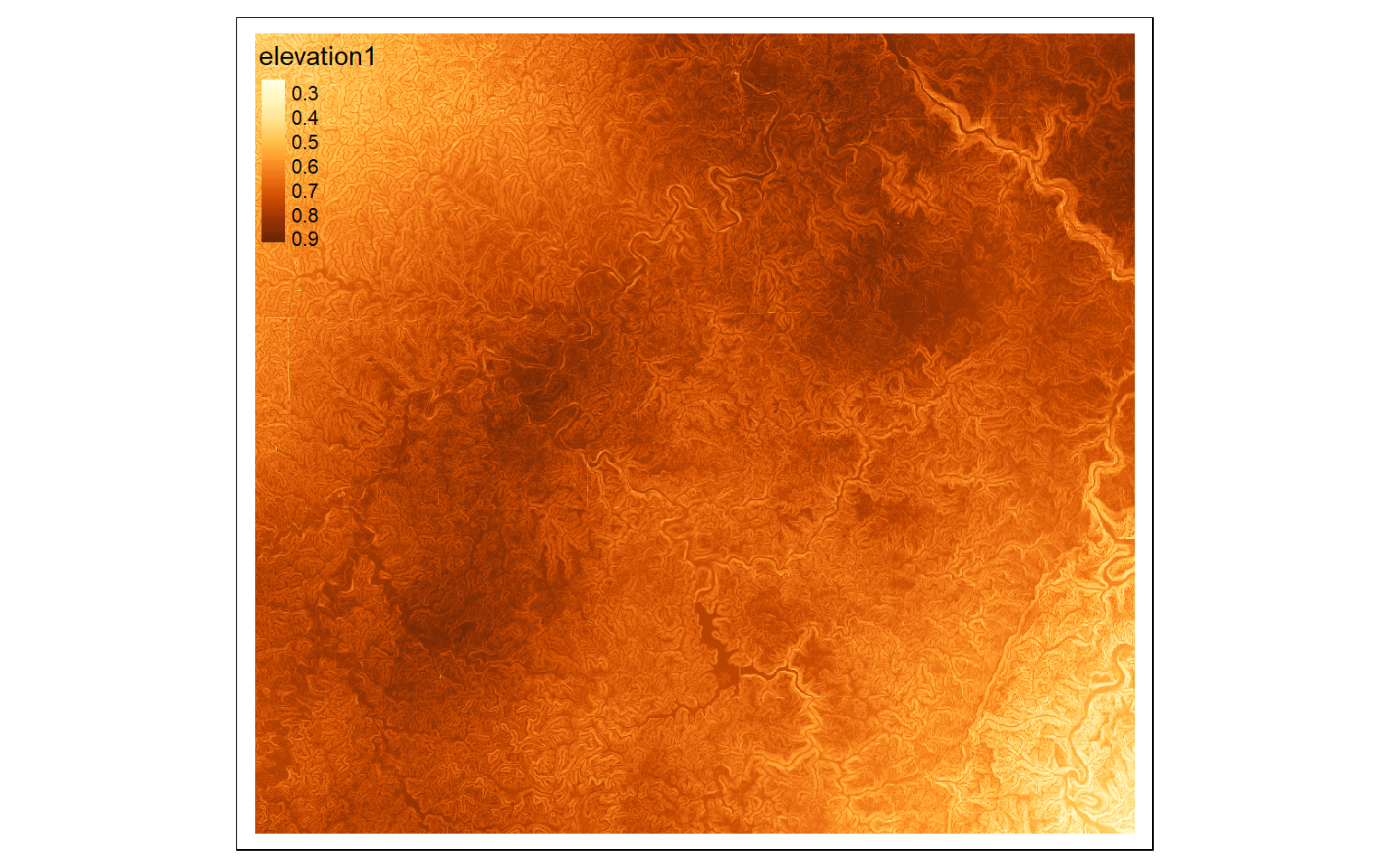

m3 <- c(0, .5, 0, .5, .6, 1, .6, 1, 2)
m3 <- matrix(m3, ncol=3, byrow = T)

wo_model_re <- classify(wo_model, m3, right=T)

tm_shape(wo_model_re)+
  tm_raster(style= "cat", labels = c("Not Suitable", "Suitable", "Very Suitable"),
            palette = c("gray", "yellow", "red"),
            title="Weight Oberlay Model")+
  tm_layout(legend.outside = TRUE)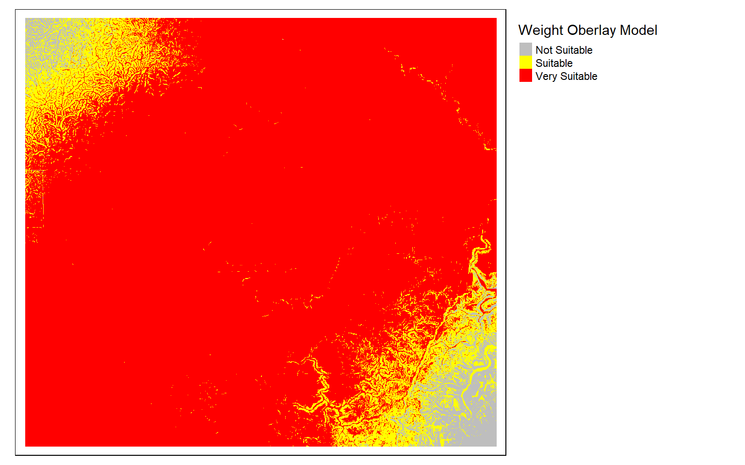

Saving Data

If you need to save an output, raster data can be saved with writeRaster() while vector data can be saved with writeVector().

Concluding Remarks

If you work with raster data in R, I highly recommend that you check out the terra package. Transitioning from the raster package is not that difficult, and terra offers significant computational and speed improvement in many cases. In short, it is worth exploring.