Working with Spatial Data
Objectives
- Read in vector data using the sp and sf packages
- Convert between the sp and sf data models
- Define and transform datums and projections for vector data
- Access and work with attribute data associated with vector features
- Read in raster data using the raster package
- Define and transform datums and projections for raster data
Overview
We are now ready to begin discussing loading, visualizing, and analyzing spatial data in R. In this section specifically, we will discuss reading in vector and raster data, working with datums and projections, and saving spatial output to disk. I will assume that you have prior knowledge of spatial data but have not worked with these data in R. If you have trouble with the theoretical components of GIScience and spatial data, we provide an additional course here focused on these topics. This course covers a variety of GIScience topics including data models, datums and projections, digital cartography, spatial analysis, and spatial modeling. The lab exercises make use of ArcGIS Pro.
Since vector and raster spatial data have fundamentally different data structures, different methods and packages are available for working with them in R. We will start with vector data.
The link at the bottom of the page provides the example data and R Markdown file used to generate this module.
Vector Data
Vector data, including points, lines, and polygons, have a more complex data structure than raster data, which is effectively an array. Within R, we need to be able to store the geographic, attribute, and coordinate system components of vector data, and there are different means to accomplish this. Initially, vector data were read into R using the sp package. More recently, the sf package has provided an alternative. I will discuss both methods here, but we will primarily focus on sf in this course.
sp
The sp package provides a variety of options for storing vector data including the following:
- SpatialPoints: stores points but no attributes
- SpatialPointsDataFrame: stores points and attributes
- SpatialLines: stores lines but no attributes
- SpatialLinesDataFrame: stores lines and attributes
- SpatialPolygons: stores polygons but no attributes
- SpatialPolygonsDataFrame: stores polygons and attributes
These data models are all subclasses of the Spatial class. This class makes use of the s4 class, in which data components are stored in slots. Let’s start by exploring this structure.
Anytime I work with spatial data in R, I load the rgdal library, which provides bindings to the Geospatial Data Abstraction Library (GDAL) and PROJ libraries. When you install these R packages the GDAL and PROJ libraries will install on your computer outside of R. Here is a link to GDAL and PROJ. I am also using the tmap package here to visualize the data in map space. We will discuss this in detail in the next section, so don’t worry if you don’t understand the syntax yet.
library(sp)
library(rgdal)
library(tmap)
Let’s build a SpatialPoints object from simulated data. First, I create a series of x, y coordinate pairs representing longitude and latitude. I then convert these data to a SpatialPoints object using the SpatialPoints() function.
When I call summary() on the new SpatialPoints object, you can see that coordinates are provided, but there is no coordinate system information defined.
pnts <- rbind(c(-79, 36), c(-101, 41), c(-80, 27), c(-91, 52), c(-68, 42))
pnts.sp <- SpatialPoints(pnts)
summary(pnts.sp)
Object of class SpatialPoints
Coordinates:
           min max
coords.x1 -101 -68
coords.x2   27  52
Is projected: NA
proj4string : [NA]
Number of points: 5
The is.projected() function can be used to test whether a projected coordinate system is defined for an object of the Spatial class. This test confirms that the projection information is missing, as NA is returned. You can use the proj4string() function on the SpatialPoints object to define a projection using a PROJ string. You can also define the projection using the European Petroleum Survey Group (EPSG) code as demonstrated in the line that is commented out. Calling summary() on the layer confirms that spatial reference information is now present. You will notice that “Is projected” is FALSE. This is because this layer is not technically “projected” since we did not use a projected coordinate system. Instead, a geographic coordinate system is defined. So, these data have been referenced to an ellipsoidal model of the Earth as opposed to a projected coordinate system.
There are many geographic and projected coordinate systems. So, you probably won’t know the EPSG code or PROJ string for a specific projection. However, you can look them up on this website. This PDF provides a great explanation of coordinate systems in R.
#Add a coordinate system
is.projected(pnts.sp)
[1] NA
proj4string(pnts.sp) <-CRS("+proj=longlat +ellps=WGS84 +datum=WGS84 +no_defs")
#proj4string(pnts.sp) <-CRS("+init=epsg:4326")
summary(pnts.sp)
Object of class SpatialPoints
Coordinates:
           min max
coords.x1 -101 -68
coords.x2   27  52
Is projected: FALSE
proj4string : [+proj=longlat +datum=WGS84 +no_defs]
Number of points: 5
We now have a SpatialPoints object. However, there is no attribute information. This is because this is not a SpatialPointsDataFrame. The next block of code demonstrates how to generate a SpatialPointsDataframe by combining SpatialPoints and a data frame. Calling summary() confirms that attributes are now present.
atts <- data.frame(attr1 = c("a", "b", "m", "l", "z"), attr2 = c(101:105),
attr3 = c("Yes", "Yes", "No", "Yes", "Yes"))
pnts.spdf <- SpatialPointsDataFrame(pnts.sp, atts)
summary(pnts.spdf)
Object of class SpatialPointsDataFrame
Coordinates:
           min max
coords.x1 -101 -68
coords.x2   27  52
Is projected: FALSE
proj4string : [+proj=longlat +datum=WGS84 +no_defs]
Number of points: 5
Data attributes:
    attr1               attr2        attr3
 Length:5           Min.   :101   Length:5
 Class :character   1st Qu.:102   Class :character
 Mode  :character   Median :103   Mode  :character
                    Mean   :103
                    3rd Qu.:104
                    Max.   :105
Generally, you will not build your spatial data from scratch. Instead, you will read spatial data into R. I will provide examples for reading in shapefile data of counties, rivers, towns, and interstates in West Virginia. This can be accomplished using the readOGR() function from the rgdal package. The dsn argument here is set to the subfolder within the working directory that houses the data. This could also be a geodatabase if you are reading in a feature class.
counties <- readOGR(dsn = "spatial_data", layer = "wv_counties")
towns <- readOGR(dsn = "spatial_data", layer = "towns")
inter <- readOGR(dsn = "spatial_data", layer = "interstates")
riv <- readOGR(dsn = "spatial_data", layer = "rivers")
I then use the tmap package to plot the data in map space. Again, we will discuss the specifics of this in the next section.
tm_shape(counties) +
tm_polygons()+
tm_shape(inter)+
tm_lines(col= "red", lwd= 2)+
tm_shape(riv)+
tm_lines(col="blue", lwd=1.5)+
tm_shape(towns)+
tm_bubbles()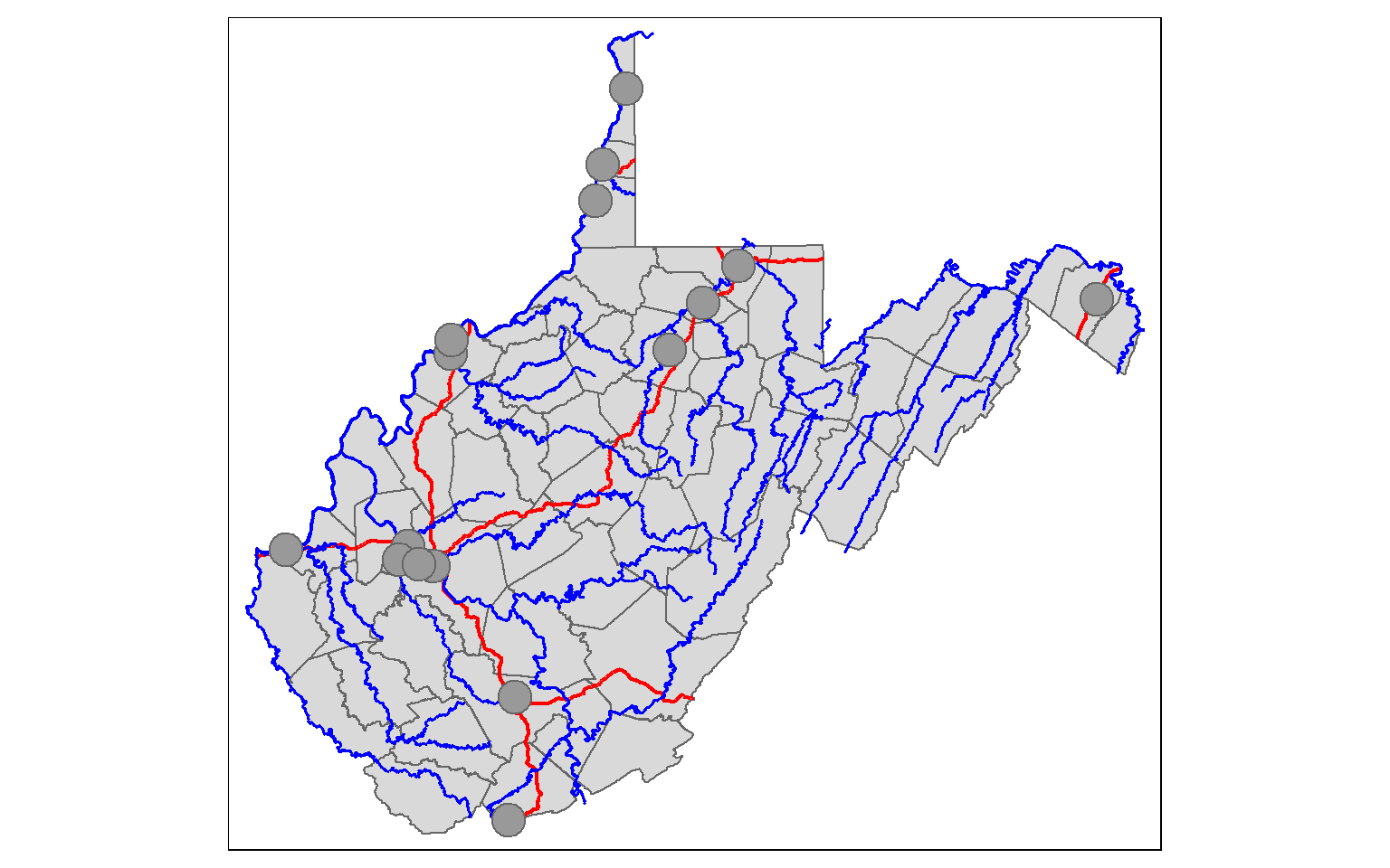
Let’s explore the data structure of the town points layer in greater detail. The s4 class and the associated Spatial subclass contain many slots. In the first line of code, I am printing the mean population by county. I have to specify the SpatialPointsDataFrame object (towns), the slot (data), and the column of interest (“POPULATION”"). Note the the data slot stores the attribute information.
mean(towns@data$POPULATION)
[1] 23100.25
The coords slot holds the coordinate pairs that define the data point locations relative to the coordinate reference system.
print(towns@coords)
      coords.x1 coords.x2
 [1,]  483651.0   4182266
 [2,]  480624.9   4123803
 [3,]  444926.6   4244910
 [4,]  557646.2   4348117
 [5,]  432818.0   4254382
 [6,]  573456.1   4370492
 [7,]  374835.7   4252617
 [8,]  760773.2   4372254
 [9,]  590140.4   4387856
[10,]  522082.3   4419227
[11,]  453171.4   4346219
[12,]  428654.7   4248147
[13,]  438223.5   4245607
[14,]  453623.5   4352732
[15,]  537004.9   4472359
[16,]  525852.3   4436142
As expected, the spatial information is more complex for a polygon. Here is an example of printing the first five coordinates that define a single polygon in the counties data set. Additional slots are available for the the ring direction, to note if holes are present, and for the area of the feature.
print(head((counties@polygons[[1]]@Polygons[[1]]@coords)))
         [,1]    [,2]
[1,] 522753.7 4431485
[2,] 522933.1 4431929
[3,] 522978.8 4432050
[4,] 523011.0 4432217
[5,] 523000.2 4432362
[6,] 522981.4 4432550
Here is an example of extracting the spatial reference information for the towns data. You can see that the spatial reference is WGS84 UTM Zone 17N.
print(proj4string(towns))
[1] "+proj=utm +zone=17 +datum=WGS84 +units=m +no_defs"
This example shows how to extract the bounding box coordinates for the data.
bbox(towns)
                min       max
coords.x1  374835.7  760773.2
coords.x2 4123803.4 4472359.3
sf
More recently, a second method has been developed for reading vector data into R. The sf package (Simple Features for R) uses a very different data structure than that used by sp as I will demonstrate here.
First, I will read in the same data layers using the st_read() function from sf.
library(sf)
counties_sf <- st_read("spatial_data/wv_counties.shp")
towns_sf <- st_read("spatial_data/towns.shp")
inter_sf <- st_read("spatial_data/interstates.shp")
riv_sf <- st_read("spatial_data/rivers.shp")
In the next code block, I run is.data.frame() on the towns_sf object, and it returns TRUE, indicating that this object is indeed a data frame. That’s weird. Actually, this object is a data frame, but how is this possible?
is.data.frame(towns_sf)
[1] TRUE
If we summarize the towns_sf object you will see that each attribute is represented as a column, and that the last column is called geometry. So, the geometric or spatial information exists as a column in the table.
summary(towns_sf)
      AREA     PERIMETER     TOWN_          TOWN_ID          TOWNS_
 Min.   :0   Min.   :0   Min.   : 17.0   Min.   : 17.0   Min.   : 17.0
 1st Qu.:0   1st Qu.:0   1st Qu.: 62.5   1st Qu.: 62.5   1st Qu.: 62.5
 Median :0   Median :0   Median :162.0   Median :162.0   Median :162.0
 Mean   :0   Mean   :0   Mean   :147.1   Mean   :147.1   Mean   :147.1
 3rd Qu.:0   3rd Qu.:0   3rd Qu.:228.0   3rd Qu.:228.0   3rd Qu.:228.0
 Max.   :0   Max.   :0   Max.   :270.0   Max.   :270.0   Max.   :270.0
    TOWNS_ID       PLACEFP              TYPE             INTPTLAT
 Min.   : 17.0   Length:16          Length:16          Length:16
 1st Qu.: 62.5   Class :character   Class :character   Class :character
 Median :162.0   Mode  :character   Mode  :character   Mode  :character
 Mean   :147.1
 3rd Qu.:228.0
 Max.   :270.0
   INTPTLNG              LAT             LONG            NAME
 Length:16          Min.   :37.26   Min.   :-82.43   Length:16
 Class :character   1st Qu.:38.37   1st Qu.:-81.65   Class :character
 Mode  :character   Median :39.27   Median :-81.20   Mode  :character
                    Mean   :38.99   Mean   :-80.95
                    3rd Qu.:39.52   3rd Qu.:-80.51
                    Max.   :40.40   Max.   :-77.97
   POPULATION       FAMILIES       HOUSEHOLDS       X_COORD
 Min.   :10753   Min.   : 2873   Min.   : 4211   Min.   :374822
 1st Qu.:12366   1st Qu.: 3453   1st Qu.: 5141   1st Qu.:443236
 Median :18178   Median : 4628   Median : 7896   Median :482122
 Mean   :23100   Mean   : 6083   Mean   : 9791   Mean   :503578
 3rd Qu.:27875   3rd Qu.: 7202   3rd Qu.:10807   3rd Qu.:542150
 Max.   :57287   Max.   :15231   Max.   :25306   Max.   :760757
    Y_COORD                 geometry
 Min.   :4123586   POINT        :16
 1st Qu.:4247294   epsg:32617   : 0
 Median :4346950   +proj=utm ...: 0
 Mean   :4315852
 3rd Qu.:4375934
 Max.   :4472140
If I print the information in this column for a single town, you can see that all the geometric information, including the geometry type, dimensions, bounding box coordinates, spatial reference information, and actual coordinates, are present. So, when using sf, vector features are read in as a data frames with a special geometry column that stores the geometric information in a list structure. This is an object-based vector data model, where the attribute and spatial information are stored in the same file. Similarly, a feature class in a geodatabase stores the geometric information in a table column as a binary large object (BLOB).
town1 <- towns_sf[1,]
print(town1$geometry)
Geometry set for 1 feature
Geometry type: POINT
Dimension:     XY
Bounding box:  xmin: 483651 ymin: 4182266 xmax: 483651 ymax: 4182266
Projected CRS: WGS 84 / UTM zone 17N
One benefit of using sf is that functions that accept data frames can also be applied to these spatial objects, since they are data frames. You will see many examples of this in the following modules.
It is possible to remove the geographic information from the data frame using st_drop_geometry(), as demonstrated in the next code block.
towns_just_attr <- st_drop_geometry(towns_sf)Conversion
Since there are two separate data models available in R for vector data, which should you use? In this course, we will primarily work with sf; however, there are many packages available for analyzing spatial data in R, and not all are able to use sf data at the time of this writing. So, it is important to be familiar with sp and also know how to convert between types. We will now discuss conversion methods.
I am reading in the towns data again using sp and sf.
towns_sp <- readOGR(dsn = "spatial_data", layer = "towns")
towns_sf <- st_read("spatial_data/towns.shp")
In this example, I am converting the sf object to sp using the as() function from sp. Setting Class to “Spatial” indicates that I want the result to be an object of class Spatial. The class() function is used to confirm this.
towns_sp_from_sf <- as(towns_sf, Class="Spatial")
class(towns_sp_from_sf)
[1] "SpatialPointsDataFrame"
attr(,"package")
[1] "sp"
Using the st_as_sf() function from sf, you can convert an object of class Spatial to a data frame, as defined by sf.
towns_sf_from_sp <- st_as_sf(towns_sp)
class(towns_sf_from_sp)
[1] "sf"         "data.frame"
Working with Vector Coordinate Systems
When working with spatial data in R, it is important that coordinate reference information be provided and that it is correctly defined. I would recommend checking the spatial reference information every time you read data into R. Using sf, projection information can be printed, written to an object, removed, or defined using the st_crs() function. In this first example, I am simply printing the projection information for the counties_sf object, which will return the EPSG code and PROJ string.
st_crs(counties_sf)
Coordinate Reference System:
  User input: WGS 84 / UTM zone 17N
  wkt:
PROJCRS["WGS 84 / UTM zone 17N",
    BASEGEOGCRS["WGS 84",
        DATUM["World Geodetic System 1984",
            ELLIPSOID["WGS 84",6378137,298.257223563,
                LENGTHUNIT["metre",1]]],
        PRIMEM["Greenwich",0,
            ANGLEUNIT["degree",0.0174532925199433]],
        ID["EPSG",4326]],
    CONVERSION["UTM zone 17N",
        METHOD["Transverse Mercator",
            ID["EPSG",9807]],
        PARAMETER["Latitude of natural origin",0,
            ANGLEUNIT["Degree",0.0174532925199433],
            ID["EPSG",8801]],
        PARAMETER["Longitude of natural origin",-81,
            ANGLEUNIT["Degree",0.0174532925199433],
            ID["EPSG",8802]],
        PARAMETER["Scale factor at natural origin",0.9996,
            SCALEUNIT["unity",1],
            ID["EPSG",8805]],
        PARAMETER["False easting",500000,
            LENGTHUNIT["metre",1],
            ID["EPSG",8806]],
        PARAMETER["False northing",0,
            LENGTHUNIT["metre",1],
            ID["EPSG",8807]]],
    CS[Cartesian,2],
        AXIS["(E)",east,
            ORDER[1],
            LENGTHUNIT["metre",1]],
        AXIS["(N)",north,
            ORDER[2],
            LENGTHUNIT["metre",1]],
    ID["EPSG",32617]]
The coordinate reference information can also be saved as a list, and individual components can be saved to vectors.
proj_info <- st_crs(counties_sf)
proj_info_proj4 <- as.vector(proj_info$proj4string)
In this example, I am removing the projection information by setting it to NA. I am then redefining the projection using the PROJ string and EPSG code.
st_crs(counties_sf) <- NA
st_crs(counties_sf)
Coordinate Reference System: NA
st_crs(counties_sf) <- "+proj=utm +zone=17 +datum=NAD83 +units=m +no_defs"
st_crs(counties_sf)
Coordinate Reference System:
  User input: +proj=utm +zone=17 +datum=NAD83 +units=m +no_defs
  wkt:
PROJCRS["unknown",
    BASEGEOGCRS["unknown",
        DATUM["North American Datum 1983",
            ELLIPSOID["GRS 1980",6378137,298.257222101,
                LENGTHUNIT["metre",1]],
            ID["EPSG",6269]],
        PRIMEM["Greenwich",0,
            ANGLEUNIT["degree",0.0174532925199433],
            ID["EPSG",8901]]],
    CONVERSION["UTM zone 17N",
        METHOD["Transverse Mercator",
            ID["EPSG",9807]],
        PARAMETER["Latitude of natural origin",0,
            ANGLEUNIT["degree",0.0174532925199433],
            ID["EPSG",8801]],
        PARAMETER["Longitude of natural origin",-81,
            ANGLEUNIT["degree",0.0174532925199433],
            ID["EPSG",8802]],
        PARAMETER["Scale factor at natural origin",0.9996,
            SCALEUNIT["unity",1],
            ID["EPSG",8805]],
        PARAMETER["False easting",500000,
            LENGTHUNIT["metre",1],
            ID["EPSG",8806]],
        PARAMETER["False northing",0,
            LENGTHUNIT["metre",1],
            ID["EPSG",8807]],
        ID["EPSG",16017]],
    CS[Cartesian,2],
        AXIS["(E)",east,
            ORDER[1],
            LENGTHUNIT["metre",1,
                ID["EPSG",9001]]],
        AXIS["(N)",north,
            ORDER[2],
            LENGTHUNIT["metre",1,
                ID["EPSG",9001]]]]
st_crs(counties_sf) <- NA
st_crs(counties_sf)
Coordinate Reference System: NA
st_crs(counties_sf) <- 26917
st_crs(counties_sf)
Coordinate Reference System:
  User input: EPSG:26917
  wkt:
PROJCRS["NAD83 / UTM zone 17N",
    BASEGEOGCRS["NAD83",
        DATUM["North American Datum 1983",
            ELLIPSOID["GRS 1980",6378137,298.257222101,
                LENGTHUNIT["metre",1]]],
        PRIMEM["Greenwich",0,
            ANGLEUNIT["degree",0.0174532925199433]],
        ID["EPSG",4269]],
    CONVERSION["UTM zone 17N",
        METHOD["Transverse Mercator",
            ID["EPSG",9807]],
        PARAMETER["Latitude of natural origin",0,
            ANGLEUNIT["degree",0.0174532925199433],
            ID["EPSG",8801]],
        PARAMETER["Longitude of natural origin",-81,
            ANGLEUNIT["degree",0.0174532925199433],
            ID["EPSG",8802]],
        PARAMETER["Scale factor at natural origin",0.9996,
            SCALEUNIT["unity",1],
            ID["EPSG",8805]],
        PARAMETER["False easting",500000,
            LENGTHUNIT["metre",1],
            ID["EPSG",8806]],
        PARAMETER["False northing",0,
            LENGTHUNIT["metre",1],
            ID["EPSG",8807]]],
    CS[Cartesian,2],
        AXIS["(E)",east,
            ORDER[1],
            LENGTHUNIT["metre",1]],
        AXIS["(N)",north,
            ORDER[2],
            LENGTHUNIT["metre",1]],
    USAGE[
        SCOPE["Engineering survey, topographic mapping."],
        AREA["North America - between 84°W and 78°W - onshore and offshore. Canada - Nunavut; Ontario; Quebec. United States (USA) - Florida; Georgia; Kentucky; Maryland; Michigan; New York; North Carolina; Ohio; Pennsylvania; South Carolina; Tennessee; Virginia; West Virginia."],
        BBOX[23.81,-84,84,-78]],
    ID["EPSG",26917]]
What if you would like to transform the datum or projection? This can be accomplished with the st_transform() function. You will need to provide the EPSG code or PROJ string for the desired output datum or projection. As an example, I am converting the county data from WGS84 UTM Zone 17N to the WGS84 geographic coordinate system.
counties_wgs84 <- st_transform(counties_sf, crs= 4236)
st_crs(counties_wgs84)
Coordinate Reference System:
  User input: EPSG:4236
  wkt:
GEOGCRS["Hu Tzu Shan 1950",
    DATUM["Hu Tzu Shan 1950",
        ELLIPSOID["International 1924",6378388,297,
            LENGTHUNIT["metre",1]]],
    PRIMEM["Greenwich",0,
        ANGLEUNIT["degree",0.0174532925199433]],
    CS[ellipsoidal,2],
        AXIS["geodetic latitude (Lat)",north,
            ORDER[1],
            ANGLEUNIT["degree",0.0174532925199433]],
        AXIS["geodetic longitude (Lon)",east,
            ORDER[2],
            ANGLEUNIT["degree",0.0174532925199433]],
    USAGE[
        SCOPE["Geodesy."],
        AREA["Taiwan, Republic of China - onshore - Taiwan Island, Penghu (Pescadores) Islands."],
        BBOX[21.87,119.25,25.34,122.06]],
    ID["EPSG",4236]]
Save to Disk
The results of your analyses in R can be saved to disk using both rgdal and sf. rgdal provides the writeORG() function which is demonstrated below. Note that you can save to a variety of vector formats; however, you must provide an object of class Spatial. So, here I am converting the data frame to the Spatial class within the writeORG() function. If you do not want to save these files to your machine, do not execute these lines of code.
writeOGR(obj=as(counties_wgs84, Class="Spatial"), dsn="spatial_data", layer="counties_wgs84", driver="ESRI Shapefile", overwrite_layer=TRUE)Data can also be exported using the st_write() function from sf. Note that I had to remove the “AREA” column since writing this field will cause an error associated with the field length.
counties_wgs84$AREA <- NULL
st_write(counties_wgs84, "spatial_data/counties_wgs84b.shp", overwrite=TRUE)
For point data, you can also save the result as a CSV file with the coordinates written to the table as demonstrated below.
st_write(towns_sf, "towns_out.csv", layer_options = "GEOMETRY=AS_XY", overwrite=TRUE)Again, I prefer to use sf to read and write vector data files in R. However, you may find sp and/or rgdal to be necessary for some tasks, so it is good to be familiar with all three packages and the associated data models.
Raster Data
As mentioned above, raster data have a simpler data structure than vector data, as these data are represented simply as an array of values. A single-band raster is similar to a matrix in R while a multi-band raster is similar to a 3-dimensional array. The primary difference between spatial raster data and other array data sets is that spatial reference information is associated with the data so that they will draw at the correct location within the map space and each cell or pixel will correspond to a certain land area. For example, a cell may cover 30-by-30 meters of land area.
Unlike vector data, there is one primary package used to work with raster grids in R: the raster package. Note that the raster package also makes use of rgdal. At the time of this writing, the new terra package is beginning to replace raster. I will cover this new package in a later module.
Raster Data Structure
To gain a better understanding of raster data, let’s build a raster grid from scratch. Using the raster() function from the raster package, I first generate an empty raster by defining the number of rows, number of columns, and the minimum and maximum coordinates in the x and y directions. I am using large numbers here because I will eventually define a UTM projection for this raster, so, easting will be reported in meters relative to the central meridian in the zone, and northing will be the distance from the equator in meters. Since the grid has 10 rows and 10 columns, there will be 100 total cells. I then create 100 random values between 0 and 255 to simulate 8-bit data using the sample() function. I set replacement equal to TRUE so that a value can be selected more than once. I then fill the empty raster with the random values using the values() function also from the raster package. The next step is to define the projection using the projection() function, again from the raster package. Here, I am using the EPSG code for WGS84 UTM Zone 17N. Lastly, I plot the raster using tmap.
library(raster)
library(rgdal)
basic_raster <- raster(ncol = 10, nrow = 10, xmn = 500000, xmx = 500100, ymn = 4200000, ymx = 4200100)
vals <- sample(c(0:255), 100, replace=TRUE)
values(basic_raster) <- vals
projection(basic_raster) <- "+init=EPSG:32617"
tm_shape(basic_raster)+
tm_raster()+
tm_layout(legend.outside = TRUE)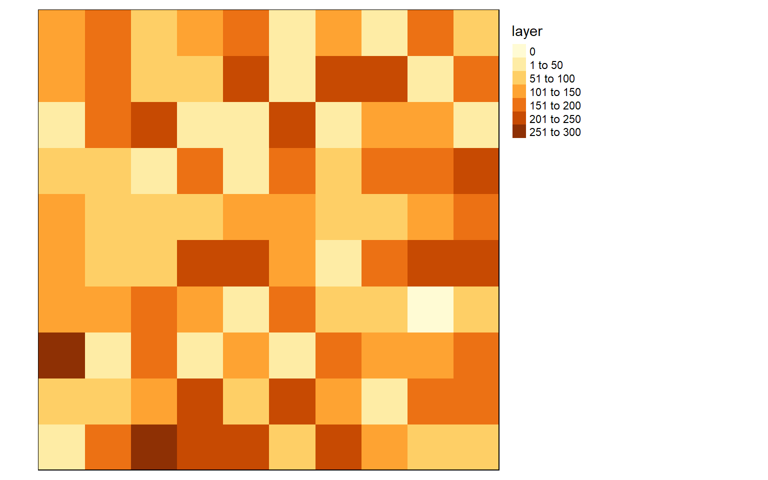
By simply typing the name of the raster into the console, information about the data is returned. It is always good to inspect the data to make sure there are no issues. The class of this object is a RasterLayer, which is defined by the raster package. It has 10 rows, 10 columns, and 100 total cells. The resolution is 10-by-10 meters. This is because we defined the extent as 100 meters of easting and northing, so each cell would need to measure 10 meters to fill the spatial extent. The EPSG code and PROJ string are provided to define the projection. The data are currently stored in memory, and the values in the cells range from 3 to 244. Note that you will probably have different values since the data were generated randomly.
basic_raster
class      : RasterLayer
dimensions : 10, 10, 100  (nrow, ncol, ncell)
resolution : 10, 10  (x, y)
extent     : 5e+05, 500100, 4200000, 4200100  (xmin, xmax, ymin, ymax)
crs        : +proj=utm +zone=17 +datum=WGS84 +units=m +no_defs
source     : memory
names      : layer
values     : 0, 254  (min, max)
Read in Single-Band Raster Data
Similar to vector data, you probably won’t create raster grids from scratch. Instead, you will read in files. We will begin with a discussion of how to read in single-band raster data.
This can be accomplished using the raster() function and calling the file name. Note that you will have to provide the entire path if the raster grid is not in your working directory. I am reading in two raster grids in the code block below. I then call the objects to inspect them. Both are projected into WGS84 UTM Zone 17N, have a cell size of 30-by-30 meters, 926 rows, 995 columns, and 921,370 total cells.
The dem layer is a digital elevation model, or DEM, while the lc layer is a land cover grid representing a portion of the National Land Cover Database (NLCD) 2011. The DEM is an example of a continuous raster grid where each cell holds a numeric measurement, in this case elevation in meters. The land cover data are an example of a categorical raster grid where each cell holds a number that is a stand-in for a category, in this case a land cover class.
#You will need to set your own working directory.
dem <- raster("spatial_data/dem_example.tif")
lc <- raster("spatial_data/lc_example.tif")
dem
class      : RasterLayer
dimensions : 928, 997, 925216  (nrow, ncol, ncell)
resolution : 30, 30  (x, y)
extent     : 619291.8, 649201.8, 4312766, 4340606  (xmin, xmax, ymin, ymax)
crs        : +proj=utm +zone=17 +datum=WGS84 +units=m +no_defs
source     : dem_example.tif
names      : dem_example
values     : 343, 1348  (min, max)
lc
class      : RasterLayer
dimensions : 928, 997, 925216  (nrow, ncol, ncell)
resolution : 29.99999, 29.99999  (x, y)
extent     : 619291.8, 649201.7, 4312766, 4340606  (xmin, xmax, ymin, ymax)
crs        : +proj=utm +zone=17 +datum=WGS84 +units=m +no_defs
source     : lc_example.tif
names      : lc_example
values     : 11, 95  (min, max)
I am now using tmap to visualize the data in map space. Note that we will talk about refining these maps in the next section. Here, I am just inspecting the data.
tm_shape(dem)+
tm_raster()+
tm_layout(legend.outside = TRUE)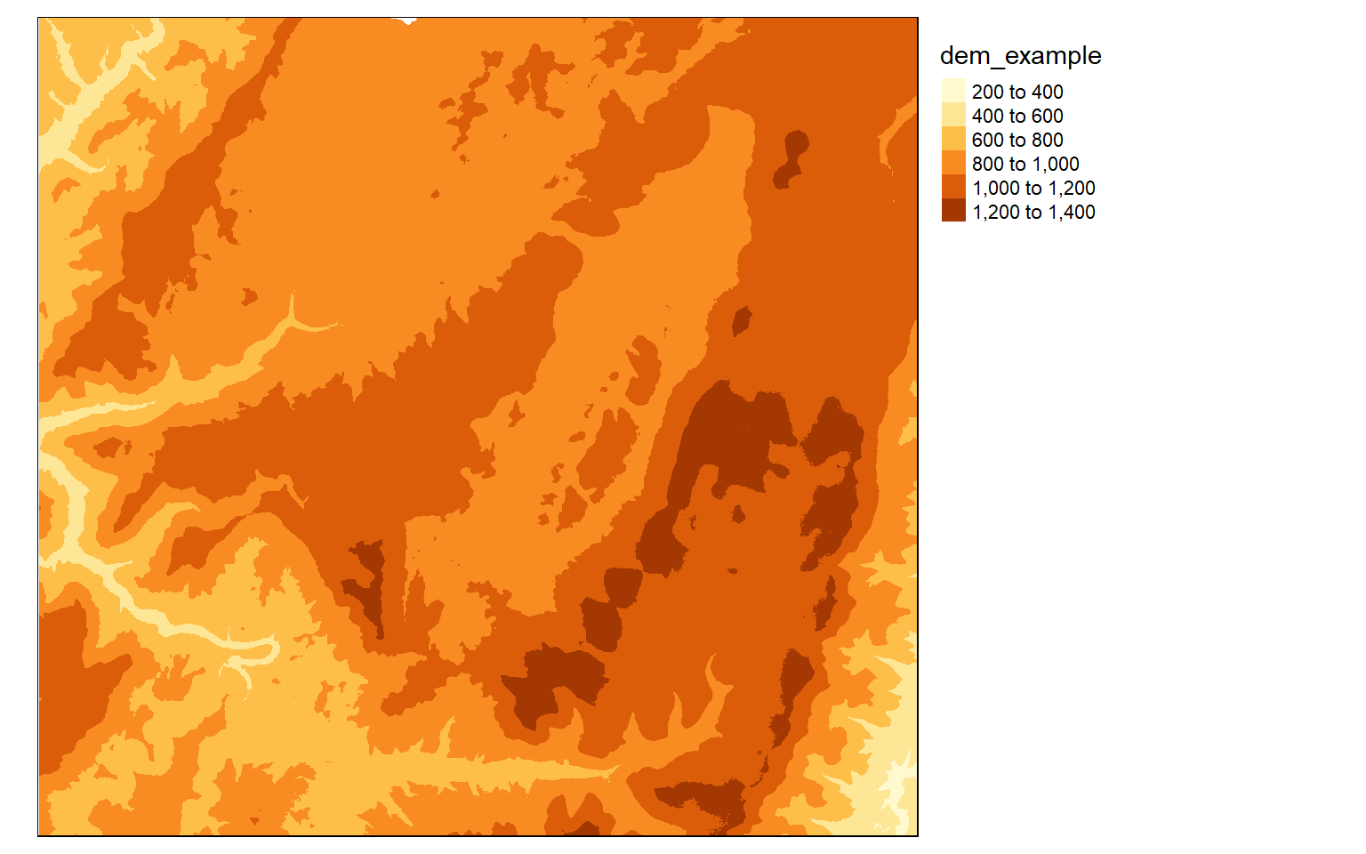
tm_shape(lc)+
tm_raster(style="cat")+
tm_layout(legend.outside = TRUE)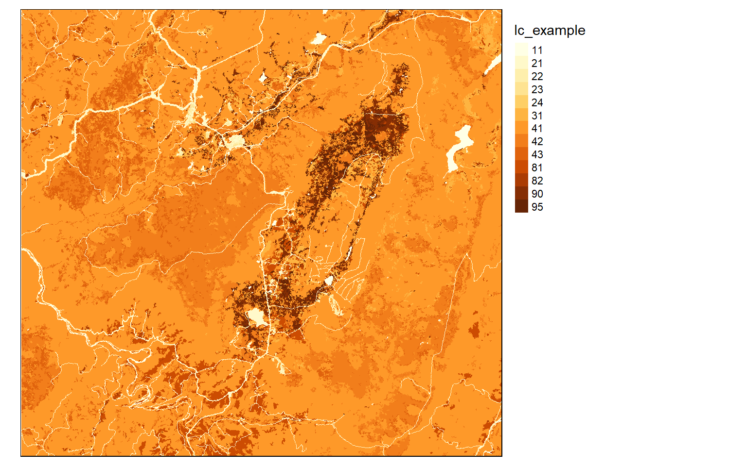
Read in Multi-Band Raster Data
To call in multi-band raster data, such as multispectral imagery, you cannot use the raster() function, as this is intended for single-band data only. Instead, you must use either brick() or stack(). A RasterBrick can only reference a single file while a RasterStack can reference multiple files or a subset of bands from one file. You can use either method to call in a multi-band file, as demonstrated in the following two examples where a Sentinel-2 multispectral image of Vancouver, British Columbia is read into R.
Note that I am using the plotRGB() function from the raster package to visualize the multi-band data as opposed to using tmap. This function allows you to specify which bands to display with each color channel and allows for contrast stretching. In the examples, the red channel is showing NIR, green is showing red, and blue is showing green. So, this is a standard false color composite where vegetated areas appear red (since they reflect a larger percentage of incoming NIR radiation).
#You will need to set your own working directory.
s1 <- brick("spatial_data/sentinel_vancouver.tif")
plotRGB(s1, r=4, g=3, b=2, stretch="lin")
#You will need to set your own working directory.
s2 <- stack("spatial_data/sentinel_vancouver.tif")
plotRGB(s1, r=4, g=3, b=2, stretch="lin")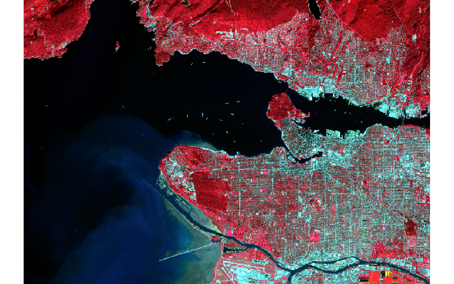
RasterBrick and RasterStack yield the same results in this case. However, if you want to reference multiple files, you cannot use a RasterBrick.
It is generally recommended to use RasterBricks when referencing a single file, as this is more computationally efficient and can speed up processing. I have found that RasterStacks may fail if all the referenced files do not have the exact same extent, number of rows, number of columns, cell size, and spatial reference system. So, I generally just stack or composite raster grids outside of R before reading them in. This is just a personal preference.
This is an example of displaying the image using histogram equalization as opposed to a linear stretch.
plotRGB(s1, r=4, g=3, b=2, stretch="hist")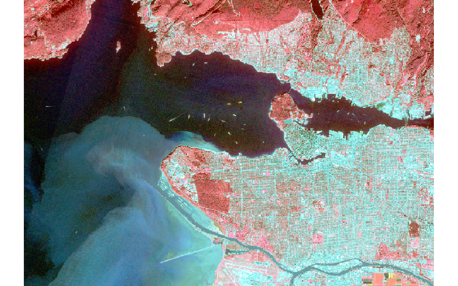
Here is an example of a different composite in which the red channel is showing shortwave infrared (SWIR), the green channel is showing NIR, and the blue channel is showing green.
plotRGB(s1, r=5, g=4, b=2, stretch="lin")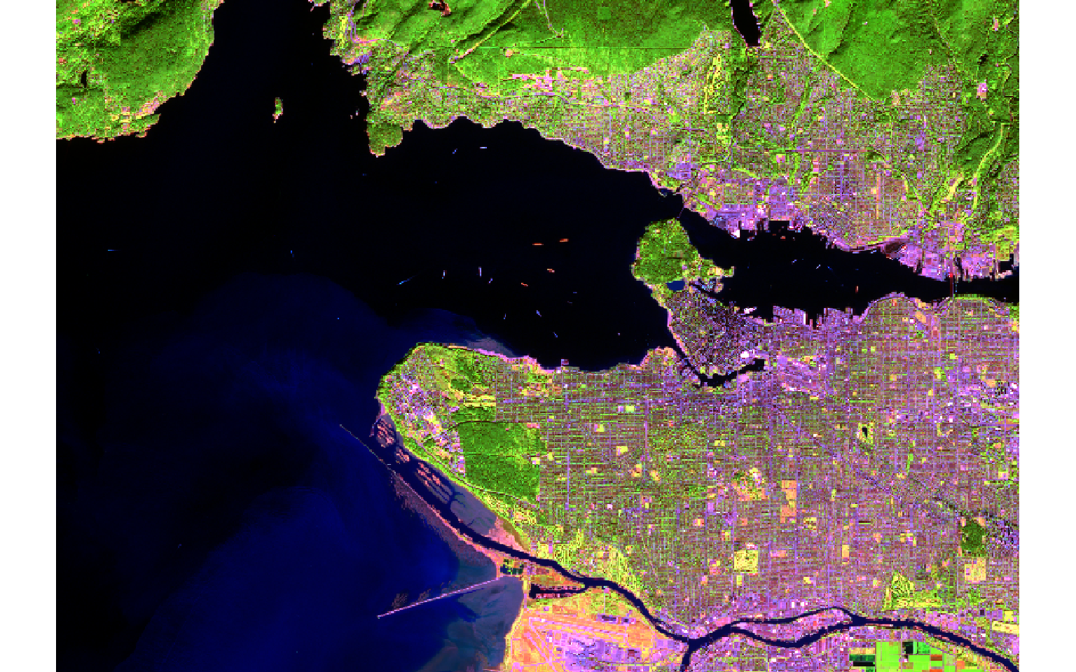
As a side note, the raster(), brick(), and stack() functions are capable of reading in any raster layer even if it does not represent geospatial data. Here is an example in which I have read in a picture of my cats: Freddy and Peri.
cats <- brick("spatial_data/example_image.tif")
plotRGB(cats, r=1, g=2, b=3)
Working with Raster Coordinate Systems
Working with raster coordinate systems is pretty similar to working with those for vector data. You can use the crs() function to obtain the projection information for a RasterLayer, RasterBrick, or RasterStack. In the example, you can see that the Sentinel-2 image is reference to WGS84 UTM Zone 10N.
crs(s1)
CRS arguments:
 +proj=utm +zone=10 +datum=WGS84 +units=m +no_defs
Similar to the example for vector data above, in this code block I am removing the spatial reference information for the Sentinel-2 data by setting it to NA. I then reapply the projection using the appropriate PROJ string. By calling crs() on this object, the projection information in returned.
crs(s1) <- NA
crs(s1)
CRS arguments: NA
crs(s1) <- "+proj=utm +zone=10 +ellps=WGS84 +towgs84=0,0,0,-0,-0,-0,0 +units=m
+no_defs"
crs(s1)
CRS arguments:
 +proj=utm +zone=10 +ellps=WGS84 +units=m +no_defs
Lastly, the projectRaster() function can be used to reproject the data into a different geographic or projected coordinate system. In the code block below I am transforming the Sentinel-2 image to the WGS84 geographic coordinate system using the corresponding EPSG code. Note that this can be slow for large data sets.
s1_wgs84 <- projectRaster(s1, crs = "+init=epsg:4236")
crs(s1_wgs84)
CRS arguments: +proj=longlat +ellps=intl +no_defs
Save to Disk
Raster data can be written to disk as a permanent file using the writeRaster() function. I generally prefer to use TIFF or IMG files when reading data in or writing data out from R. However, a variety of formats are available and can be specified using the format argument.
writeRaster(s1_wgs84, filename="s1_wgs84", format = "GTiff", overwrite=TRUE)Concluding Remarks
Now that you know how to read in geospatial data in R and the characteristics of the data models used to represent vector and raster data, you can start using these data in your analyses. In the next section, we will explore visualizing spatial data using the tmap package. In later sections, we will explore vector- and raster-based spatial analysis.