Machine Learning with Random Forest
Objectives
- Create predictive models using the random forest (RF) algorithm and the randomForest package
- Predict to validation data to assess model performance
- Predict to raster data to make spatial predictions
- Assess variable importance
- Assess models using receiver operating characteristic curves (ROC) and the area under the curve (AUC) measure
Overview
Before we experiment with using the caret package, which provides access to a variety of different machine learning algorithms, in this module we will explore the randomForest package to implement the random forest (RF) algorithm specifically. I will step through the process of creating a spatial prediction to map the likelihood or probability of palustrine forested/palustrine scrub/shrub (PFO/PSS) wetland occurrence using a variety of terrain variables. The provided training.csv table contains 1,000 examples of PFO/PSS wetlands and 1,000 not PFO/PSS examples. The validation.csv file contains a separate, non-overlapping 2,000 examples equally split between PFO/PSS wetlands and not PFO/PSS wetlands. I have also provided a raster stack (predictors.img) of all the predictor variables so that a spatial prediction can be produced. Since PFO/PSS wetlands should only occur in woody or forested extents, I have also provided a binary raster mask (for_mask.img) to subset the final result to only these areas. The link at the bottom of the page provides the example data and R Markdown file used to generate this module.
Here is a brief description of all the provided variables.
- class: PFO/PSS (wet) or not (not)
- cost: Distance from water bodies weighted by slope
- crv_arc: Topographic curvature
- crv_plane: Plan curvature
- crv_pro: Profile curvature
- ctmi: Compound topographic moisture index (CTMI)
- diss_5: Terrain dissection (11 x 11 window)
- diss_10: Terrain dissection (21 x 21 window)
- diss_20: Terrain dissection (41 x 41 window)
- diss_25: Terrain dissection (51 x 51 window)
- diss_a: Terrain dissection average
- rough_5: Terrain roughness (11 x 11 window)
- rough_10: Terrain roughness (21 x 21 window)
- rough_20: Terrain roughness (41 x 41 window)
- rough_25: Terrain Roughness (51 x 51 window)
- rough_a: Terrain roughness average
- slp_d: Topographic slope in degrees
- sp_5: Slope position (11 x 11 window)
- sp_10: Slope position (21 x 21 window)
- sp_20: Slope position (41 x 41 window)
- sp_25: slope position (51 x 51 window)
- sp_a: Slope position average
The data provided in this example are a subset of the data used in this publication:
Maxwell, A.E., T.A. Warner, and M.P. Strager, 2016. Predicting palustrine wetland probability using random forest machine learning and digital elevation data-derived terrain variables, Photogrammetric Engineering & Remote Sensing, 82(6): 437-447. https://doi.org/10.1016/S0099-1112(16)82038-8.
As always, to get started I am reading in all of the needed packages and data. The tables are read in using read.csv() and the raster data are loaded using the raster() function from the raster package. I created the training data by extracting raster data values at point locations using GIS software. I then saved the tables to CSV files. This process could also be completed in R using methods we have already discussed.
I then rename the raster bands to match the column names from the table. Note that the band order doesn’t matter; however, the correct name must be associated with the correct variable or band.
require(randomForest)
require(pROC)
require(raster)
require(rgdal)
require(tmap)
require(ggplot2)
require(caret)
train <- read.csv("random_forests/training.csv", sep=",", header=TRUE, stringsAsFactors=TRUE)
test <- read.csv("random_forests/validation.csv", sep=",", header=TRUE, stringsAsFactors=TRUE)
preds <- brick("random_forests/predictors.tif")
mask <- raster("random_forests/for_mask.tif")names(preds) <- c("cost", "crv_arc", "crv_plane", "crv_pro", "ctmi", "diss_5", "diss_10", "diss_20", "diss_25", "diss_a", "rough_5", "rough_10", "rough_20", "rough_25", "rough_a", "slp_d", "sp_5", "sp_10", "sp_20", "sp_25", "sp_a") Create the Model
The code block below shows how to train a model with the randomForest() function from the randomForest package. The first column in the table (“class”) is the dependent variable while columns 2 through 22 provide the predictor variables. I am using 501 trees, calculating measures of variable importance, and assessing the model using the out of bag (OOB) data with a confusion matrix and an error rate. I am also setting a random seed to make sure that the results are reproducible.
set.seed(42)
rf_model <- randomForest(y= train[,1], train[,2:22], ntree=501, importance=T, confusion=T, err.rate=T)
Once the model is produced, I call it to print a summary of the results. The model generally performed well. The OOB error rate was only 3.2%, or 96.8% of the OOB data were correctly classified. Of the PFO/PSS samples, only 26 were incorrectly classified while 38 of the not wetland class were incorrectly classified, so omission and commission error are nearly balanced. You can also see that the algorithm used 4 random variables for splitting at each node (the mtry parameter). Since I did not specify this, the square root of the number of predictor variables was used.
rf_model

Call:
 randomForest(x = train[, 2:22], y = train[, 1], ntree = 501,      importance = T, confusion = T, err.rate = T)
               Type of random forest: classification
                     Number of trees: 501
No. of variables tried at each split: 4

        OOB estimate of  error rate: 3.2%
Confusion matrix:
    not wet class.error
not 962  38       0.038
wet  26 974       0.026
Variable Importance
Using the importance() function from the randomForest package, we can obtained the importance estimates for each variable relative to each class and also overall using the OOB mean decrease in accuracy and/or mean decrease in Gini measures. In the second code block, I have plotted the importance measures. Higher values indicate a greater importance in the model.
Note that random forest-based importance measures have been shown to be biased if predictor variables are highly correlated, variables are measured on different scales, a mix of continuous and categorical variables are used, and/or categorical variables have varying numbers of levels. In this example, variables are very correlated since we calculated the same measures at different window sizes, so this is an issue. The party and perimp packages provide measures of conditional variable importance, which can be used to assess importance while taking into account variable correlation. Further, this package allows for approximations of both partial (i.e., conditional) and marginal importance. Partial importance relates to importance of a variable within the feature space and takes into account correlation between variables while marginal importance assess the relationship between the dependent variable and variable of interest without taking into account the other predictor variables in the model. With no correlation between predictor variables, partial and marginal importance are equivalent. Another means to assess variable importance using the RF algorithm is made available in the Boruta package. You may also want to check out the rfUtilities package.
Documentation for the party package can be found here. Here is a link to a paper on this topic by Strobl et al. Documentation for Boruta can be found here while a research article introducing the method can be found here.
importance(rf_model)
                 not       wet MeanDecreaseAccuracy MeanDecreaseGini
cost       9.5252422 26.627942            26.913251       183.188275
ctmi       2.7114363  8.134470             8.741014         6.663290
crv_arc    0.8500137 10.510031            10.452762         4.759517
crv_plane  0.6693872 14.716239            14.389290         6.121970
crv_pro    1.6327988  8.709588             9.024416         4.449532
diss_10   14.0786011 15.869143            18.687559        32.797680
diss_20   15.5952264 17.916204            21.615596        64.318851
diss_25   18.5173809 19.342369            25.875810        79.512844
diss_5     7.7825581 13.160540            12.544342        11.840202
diss_a    11.2746311 15.828505            17.357294        31.550745
rough_10  12.2591646 17.233047            20.542069        86.359892
rough_20  14.3058916 13.788886            19.369884        51.784669
rough_25  16.5848323 12.871523            20.772291        42.153341
rough_5   10.8049583 16.728945            19.350248       136.217674
rough_a   12.4748354 15.021272            19.195641        68.487471
slp_d      9.9272365 11.959671            15.787975       125.113741
sp_10      8.5270362 12.050580            14.824608        10.423877
sp_20      9.5984981 12.731844            14.887266        13.122625
sp_25      6.4062282 14.352896            15.471995        18.392499
sp_5       8.9935641 12.050825            14.461741         8.129591
sp_a 8.7554578 13.501101 15.947827 14.138012varImpPlot(rf_model)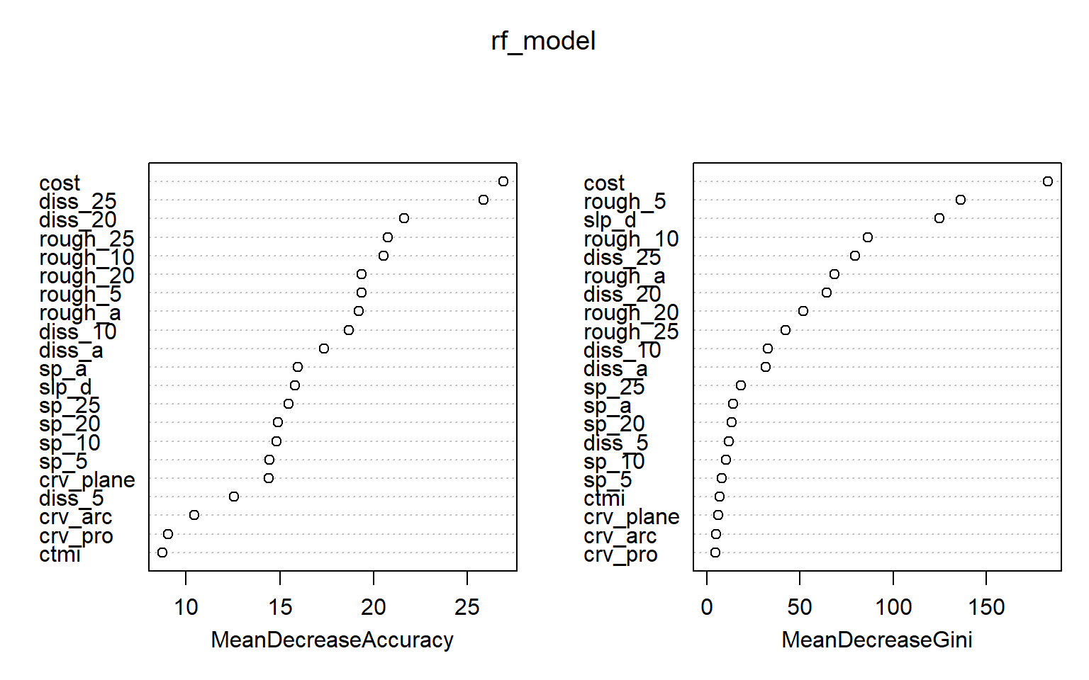
Calling plot() on the random forest model object will show how OOB error changes with the number of trees in the forest. This plot suggests that the model stabilizes after roughly 100 trees. I generally use 500 or more trees, as it has been shown that using more trees generally doesn’t reduce classification accuracy or cause overfitting. However, more trees will make the model more computationally intensive. If you aren’t sure how many trees to build, you can use this plot to assess the impact.
plot(rf_model)
Partial dependency plots are used to assess the dependency or response of the model to a single predictor variable. In the following examples, I have created plots to assess the impact of topographic slope, cost distance from streams weighted by topographic slope, and topographic dissection calculated with a 25-by-25 cell circular radius window size. The function requires that a model, data set, predictor variable of interest, and class of interest are provided. To generate these plots, the variable of interest is maintained in the model while the mean value is used for all other variables. Generally, lower slopes, proximity to streams, and more incision or dissection seem to be correlated with wetland occurrence. Although these graphs can be informative, they can also be noisy. So, be careful about reading too much into noisy patterns.
partialPlot(x=rf_model, pred.data=train, x.var=slp_d, which.class="wet")
partialPlot(x=rf_model, pred.data=train, x.var=cost, which.class="wet")
partialPlot(x=rf_model, pred.data=train, x.var=diss_25, which.class="wet")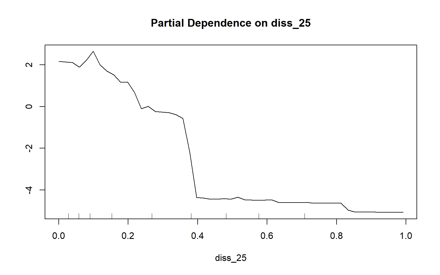
Prediction and Assessment
Now that we have a model, it can be used to predict to new data. In the next code block, I am predicting to the test or validation data. Instead of obtaining the resulting binary classification, I am using type=“prob” to obtain the resulting class likelihood or probability. Using type=“class” will return the classification result. I am setting the index equal to 2, since I want the probability for the wetland class as opposed to the not class. Generally, the values are indexed alphabetically. If norm.votes is TRUE then the class votes will be expressed as a fraction as opposed to a count. With predict.all set to FALSE, all predictions will not be written out, only the final result. When proximity is equal to FALSE, proximity measures will not be computed. When the nodes argument is set to FALSE a matrix of terminal node indicators will not be written to the result. So, I am simply obtaining the final probability value for each class with no additional information. Calling head() on the result will show the probability for the first five samples scaled from 0 to 1.
pred_test <- predict(rf_model, test, index=2, type="prob", norm.votes=TRUE, predict.all=FALSE, proximity=FALSE, nodes=FALSE)
head(pred_test)
Output:            not       wet
Output:  1 0.001996008 0.9980040
Output:  2 0.035928144 0.9640719
Output:  3 0.001996008 0.9980040
Output:  4 0.003992016 0.9960080
Output:  5 0.001996008 0.9980040
Output:  6 0.000000000 1.0000000
To assess the model, I am now producing an ROC curve and associated AUC value using the roc() function from the pROC package. This requires that the correct class and resulting prediction be provided. An AUC value of 0.991 is obtained, suggesting strong model performance.
pred_test <- data.frame(pred_test)
pred_test_roc <- roc(test$class, pred_test$wet)
auc(pred_test_roc)
Area under the curve: 0.9912
plot(pred_test_roc)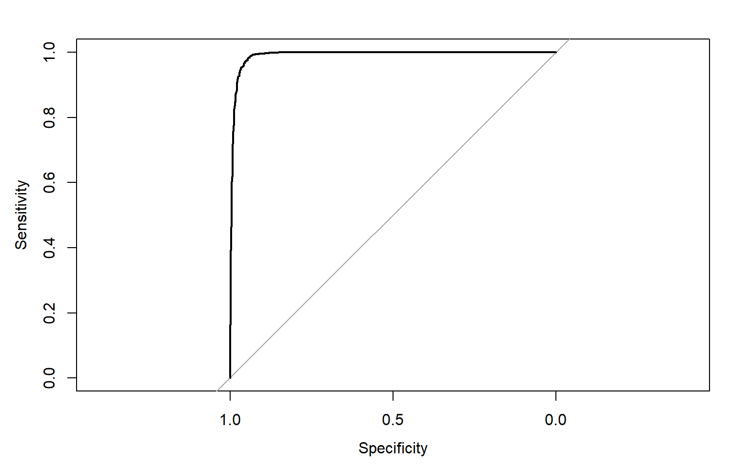
ROC curves can also be plotted using ggplot2 and the ggroc() function. This is my preferred method, as it allows for the customization options of ggplot2 to be applied. You can also plot ROC curves for multiple models to the same graph for comparison, as will be demonstrated below. I have also plotted the reference line using geom_abline() with an intercept of 1 and a slope of 1.
ggroc(pred_test_roc, lwd=1.2, col="blue")+
geom_abline(intercept = 1, slope = 1, color = "red", linetype = "dashed", lwd=1.2)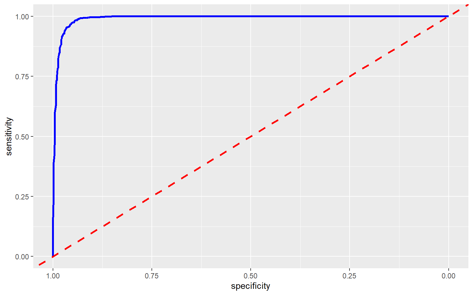
Predicting to a raster grid is very similar to predicting to a table. I am providing the raster data and the trained model. I am also indicating that I want the probability of PFO/PSS wetland occurrence to be written out to each cell using type=“prob” and index=2. I am providing a file name for the raster output. If a full file path is not provided, then the grid will be written to the current working directory. I would recommend saving to TIFF or IMG format. Setting progress equal to “window” will cause a progress window to be launched. This can be useful since making predictions at every cell in a raster grid stack can take some time. Remember that the correct variable name must be assigned to each band. Also, it is okay to include bands that won’t be used. They are simply ignored.
predict(preds, rf_model, type="prob", index=2, na.rm=TRUE, progress="window", overwrite=TRUE, filename="random_forests/rf_wetland.img")Once the model is created, I then read it back in using the raster() function, since it is a single-band raster. I then multiply the result by the mask so that all areas that are not woody are no longer predicted. Lastly, I create a map of the output using tmap. Generally, areas in low topographic positions near streams are predicted to be more likely to be wetlands than other topographic positions, which makes sense.
raster_result <- raster("random_forests/rf_wetland.img")
masked_result <- mask*raster_resulttm_shape(masked_result)+
tm_raster(palette="Blues")+
tm_layout(legend.outside = TRUE)+
tm_layout(title = "Wetland Probability", title.size = 1.5)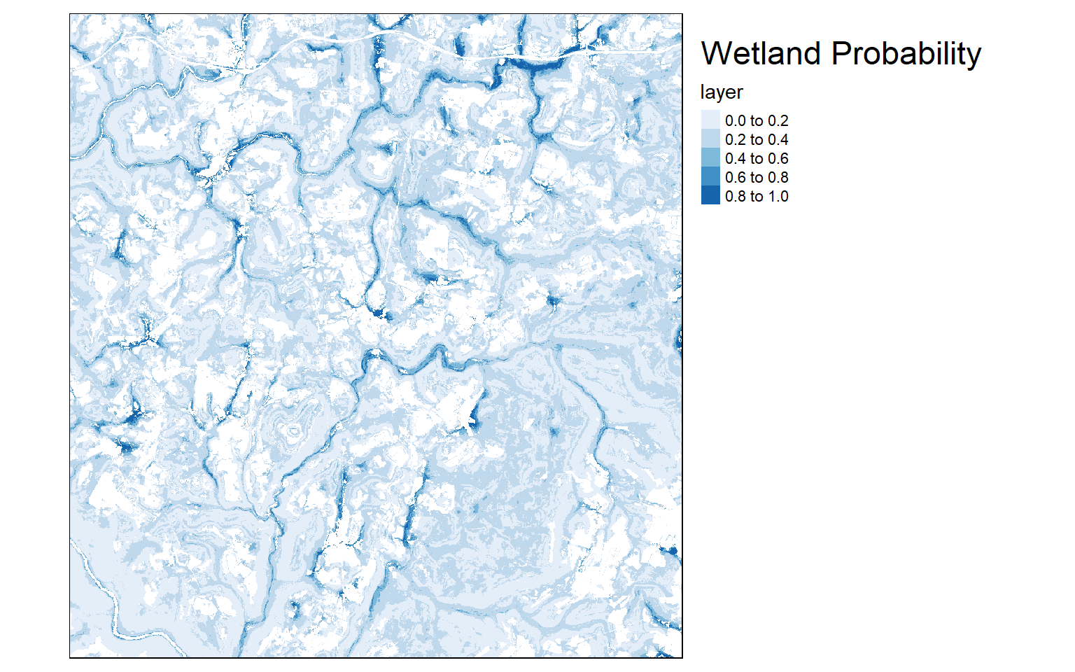
If you would like to assess the model using the binary classification as opposed to the class probabilities, you will need to change the type to “class” when predicting to new data. In this example, I am predicting out the class for each validation or test sample. I then use the confusionMatrix() function from caret to generate a confusion matrix. This function requires that the predicted and correct class be provided. I am also specifying that “wet” represents the positive case. The mode argument allows you to control what measures are provided. The options include “sens_spec”, “prec_recall”, or “everything.” When using “everything”, a wide variety of measures are provided including specificity, sensitivity, precision, recall, and F1 score. The results suggest strong performance, with a 96.4% accuracy and a Kappa statistic of 0.927. Precision and recall are both above 0.95.
Although I will not demonstrate it here, diffeR is another great package for assessing models. The documentation for this package can be found here.
pred_test_class <- predict(rf_model, test, type="class", norm.votes=TRUE, predict.all=FALSE, proximity=FALSE, nodes=FALSE)
head(pred_test_class)
  1   2   3   4   5   6
wet wet wet wet wet wet
Levels: not wetconfusionMatrix(pred_test_class, test$class, positive="wet", mode="everything")
Confusion Matrix and Statistics
Reference
Prediction not wet
not 946 22
wet 54 978
Accuracy : 0.962
95% CI : (0.9527, 0.9699)
No Information Rate : 0.5
P-Value [Acc > NIR] : < 2.2e-16
Kappa : 0.924
Mcnemar's Test P-Value : 0.0003766
Sensitivity : 0.9780
Specificity : 0.9460
Pos Pred Value : 0.9477
Neg Pred Value : 0.9773
Precision : 0.9477
Recall : 0.9780
F1 : 0.9626
Prevalence : 0.5000
Detection Rate : 0.4890
Detection Prevalence : 0.5160
Balanced Accuracy : 0.9620
'Positive' Class : wet
ROC curves and the AUC measure can be used to compare models. In the next two code blocks I create models using just topographic slope followed by just the compound topographic moisture index (CTMI). The slope-only model provides an AUC of 0.934 while the CTMI-only model results in an AUC of 0.776, suggesting that CTMI is less predictive of wetland occurrence than topographic slope.
set.seed(42)
rf_model_slp <- randomForest(class~slp_d, data=train, ntree=501, importance=T, confusion=T, err.rate=T)
pred_test_slp <- predict(rf_model_slp, test, index=2, type="prob", norm.votes=TRUE, predict.all=FALSE, proximity=FALSE, nodes=FALSE)
pred_test_slp <- data.frame(pred_test_slp)
pred_test_slp_roc <- roc(test$class, pred_test_slp$wet)
auc(pred_test_slp_roc)
Area under the curve: 0.9337set.seed(42)
rf_model_ctmi <- randomForest(class~ctmi, data=train, ntree=501, importance=T, confusion=T, err.rate=T)
pred_test_ctmi <- predict(rf_model_ctmi, test, index=2, type="prob", norm.votes=TRUE, predict.all=FALSE, proximity=FALSE, nodes=FALSE)
pred_test_ctmi <- data.frame(pred_test_ctmi)
pred_test_ctmi_roc <- roc(test$class, pred_test_ctmi$wet)
auc(pred_test_ctmi_roc)
Area under the curve: 0.7755It is also possible to plot multiple ROC curves in the same space using the ggroc() function from ggplot2 by providing a list of ROC results. This provides an informative comparison of the three models produced in this exercise. Also, this allows for the customization provided by ggplot2.
ggroc(list(All=pred_test_roc, Slp=pred_test_slp_roc, ctmi=pred_test_ctmi_roc), lwd=1.2)+
geom_abline(intercept = 1, slope = 1, color = "red", linetype = "dashed", lwd=1.2)+
scale_color_manual(labels = c("All Variables", "Just CTMI", "Just Slope"), values= c("#88D04B", "#D65076", "#EFC050"))+
ggtitle("Model Comparison")+
labs(x="Specificity", y="Sensitivity")+
theme(axis.text.y = element_text(size=12))+
theme(axis.text.x = element_text(size=12))+
theme(plot.title = element_text(face="bold", size=18))+
theme(axis.title = element_text(size=14))+
theme(strip.text = element_text(size = 14))+
theme(legend.title=element_blank())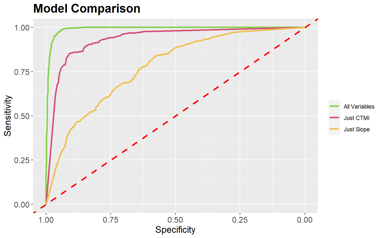
The pROC package also provides a statistical test to compare ROC curves (the DeLong Test). In the example, I am comparing the original model, with all predictor variables, to the model using only the topographic slope variable. This test suggests statistical difference, or that the model with all terrain features is providing a better prediction than the one using just slope.
roc.test(pred_test_roc, pred_test_slp_roc)

    DeLong's test for two correlated ROC curves

data:  pred_test_roc and pred_test_slp_roc
Z = 10.968, p-value < 2.2e-16
alternative hypothesis: true difference in AUC is not equal to 0
95 percent confidence interval:
 0.04719219 0.06772881
sample estimates:
AUC of roc1 AUC of roc2
  0.9911565   0.9336960
Concluding Remarks
I hope that this module provided an informative introduction to machine learning in R using the randomForest package. In the next module, we will explore the caret package for implementing a variety of machine learning algorithms in R to make a wide variety of predictions.