Raster-Based Spatial Analysis in R
Objectives
- Process raster data including changing the cell size, spatial extent, and cell values
- Perform raster math and calculations
- Generate distance and density grid surfaces
- Produce conservative or binary models
- Create liberal models using weighted overlay
- Work with the raster package
Overview
In this section we will focus on working with raster geospatial data in R. We will primarily rely on the raster package since it is currently the dominant method for handling and analyzing raster data. In the next module, I will demonstrate the new terra package that will eventually replace raster. Similar to the last module, we will visualize the results using tmap. In the first code block, I am calling in the required packages.
library(sf)
library(rgdal)
library(raster)
library(tmap)
library(tmaptools)
library(spatialEco)
library(RStoolbox)
In this module, we will work with data from West Virginia. Here is a brief description of the data. The link at the bottom of the page provides the example data and R Markdown file used to generate this module.
- elev: 30 m resolution digital elevation model (DEM) in meters from the National Elevation Dataset (NED)
- slp: slope in degrees derived from the elevation raster grid
- lc: 30 m resolution categorical land cover grid from the 2011 National Land Cover Database (NLCD)
- airports: airports in West Virginia
- pnts: random points
- ws: watershed boundaries for subset of the state
- str: man-made structures mapped as points for portion of the state
All raster grids are being read using the raster() function from the raster package, as they are all single-band raster grids. The vector geospatial data are being read using st_read() from the sf package. All raster data are in TIFF format while all vector data are stored as shapefiles. I also map the DEM to check that it has loaded correctly. I recommend checking your data prior to any analyses.
elev <- raster("raster_analysis/elevation1.tif")
slp <- raster("raster_analysis/slope1.tif")
lc <- raster("raster_analysis/lc_example.tif")
airports <- st_read("raster_analysis/airports.shp")
interstates <- st_read("raster_analysis/interstates.shp")
pnts <- st_read("raster_analysis/example_points.shp")
ws <- st_read("raster_analysis/watersheds.shp")
str <- st_read("raster_analysis/structures.shp")tm_shape(elev)+
tm_raster(style= "cont")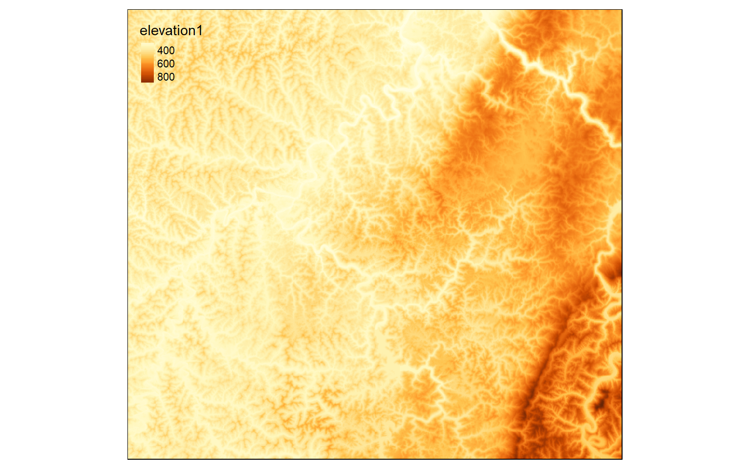
Crop, Merge, and Mask
A common pre-processing task is to extract out a spatial subset of a raster grid. In R, this can be accomplished using a variety of methods from the raster package. In the first code block below I am defining a rectangular extent by providing the desired xmin, xmax, ymin, and ymax values relative to the projection of the data (WGS84 UTM Zone 17N) using the extent() function from the raster package.
In the next set of code I am using the crop() function to extract out all the cells within the defined extent. By calling the result, I can inspect the number of rows and columns, spatial resolution, number of bands, and projection information. Note that this raster grid is being stored in memory. Lastly, I plot the cropped extent.
crop_extent <- extent(580000, 620000, 4350000, 4370000)elev_crop <- crop(elev, crop_extent)
elev_crop
class : RasterLayer
dimensions : 667, 1164, 776388 (nrow, ncol, ncell)
resolution : 30, 30 (x, y)
extent : 579997.6, 614917.6, 4350005, 4370015 (xmin, xmax, ymin, ymax)
crs : +proj=utm +zone=17 +datum=WGS84 +units=m +no_defs
source : memory
names : elevation1
values : 287, 896 (min, max)
tm_shape(elev_crop)+
tm_raster(style= "cont")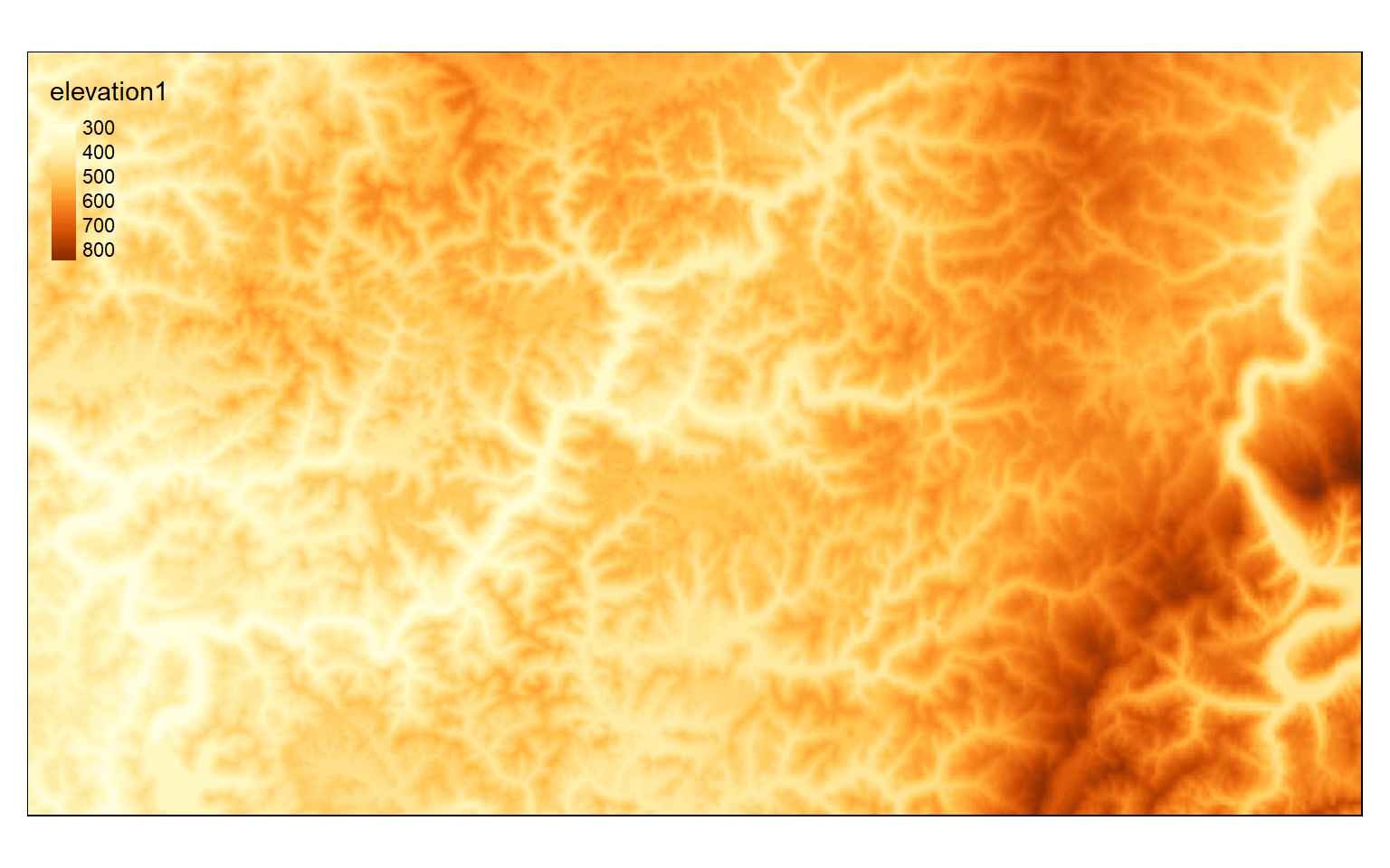
Other than cropping a raster grid using a defined rectangular extent, you can also extract based on row and column numbers. As an example, I am extracting out columns 500 through 600 and rows 400 through 800. Note that the syntax here is a bit different from the example above, as you will need to call the raster grid inside of extent(). This method is useful if you want to remove the margin rows and columns of a raster grid.
elev_crop2 <- crop(elev_crop, extent(elev_crop, 500,600,400, 800))
elev_crop2
class : RasterLayer
dimensions : 101, 401, 40501 (nrow, ncol, ncell)
resolution : 30, 30 (x, y)
extent : 591967.6, 603997.6, 4352015, 4355045 (xmin, xmax, ymin, ymax)
crs : +proj=utm +zone=17 +datum=WGS84 +units=m +no_defs
source : memory
names : elevation1
values : 359, 617 (min, max)
tm_shape(elev_crop2)+
tm_raster(style= "cont")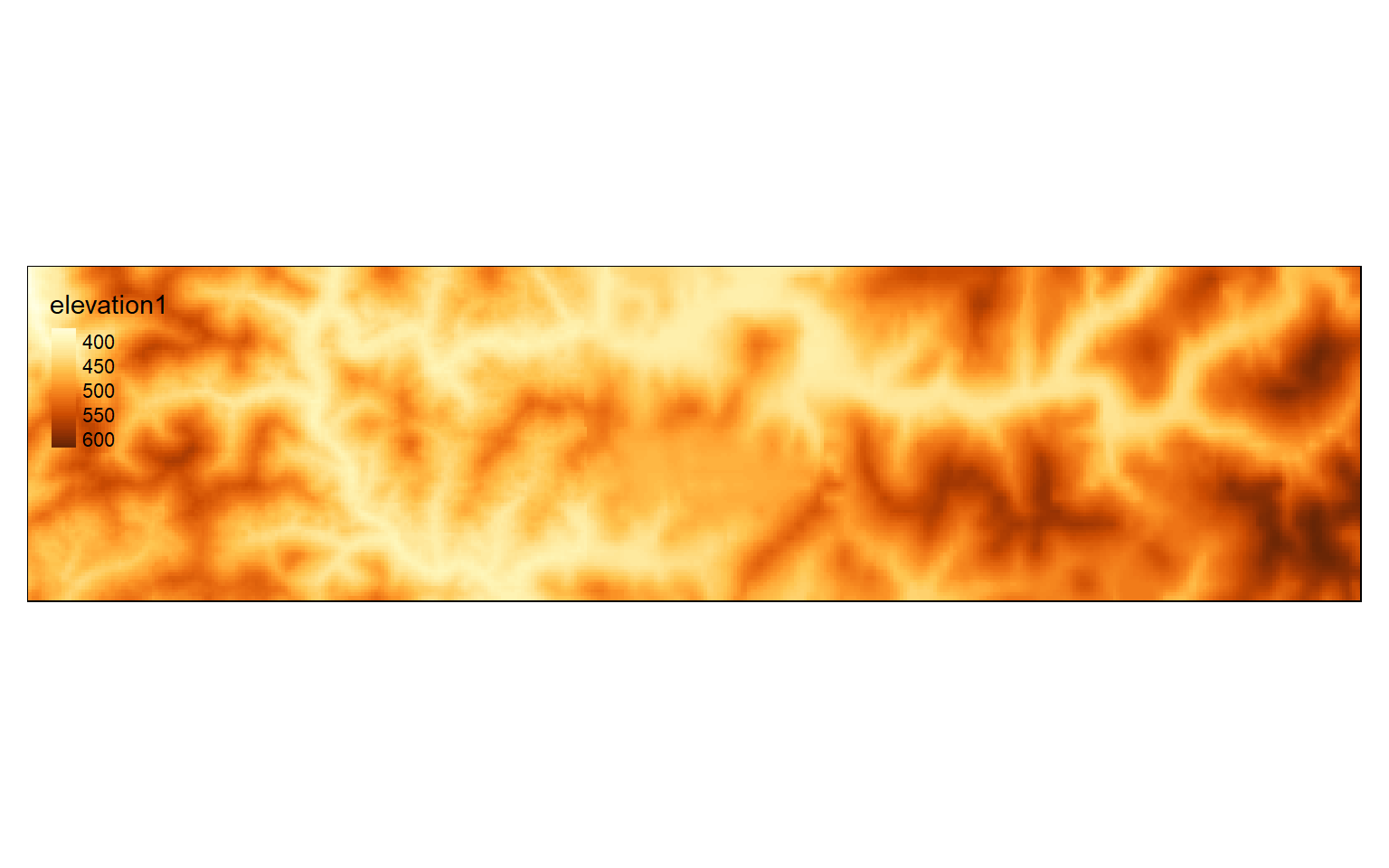
Other than extracting out a subset of the data, you can also merge multiple raster grids into a single object using the merge() function. To demonstrate this, I first extract a different spatial extent so that I have two grids to merge that partially overlap. I then use the merge() function to combine or mosaic the two grids. Lastly, I map the result.
elev_crop3 <- crop(elev_crop, extent(elev_crop, 550, 700, 500, 900))
elev_crop3
class : RasterLayer
dimensions : 118, 401, 47318 (nrow, ncol, ncell)
resolution : 30, 30 (x, y)
extent : 594967.6, 606997.6, 4350005, 4353545 (xmin, xmax, ymin, ymax)
crs : +proj=utm +zone=17 +datum=WGS84 +units=m +no_defs
source : memory
names : elevation1
values : 393, 834 (min, max)
tm_shape(elev_crop3)+
tm_raster(style= "cont")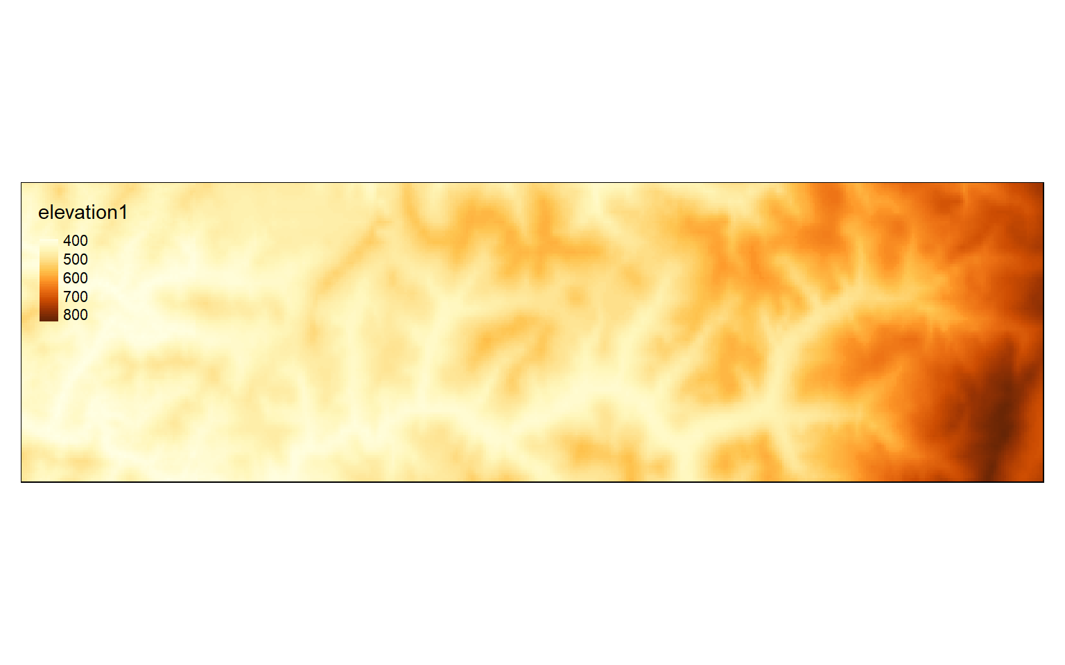
elev_merge <- merge(elev_crop2, elev_crop3)
tm_shape(elev_merge)+
tm_raster(style= "cont")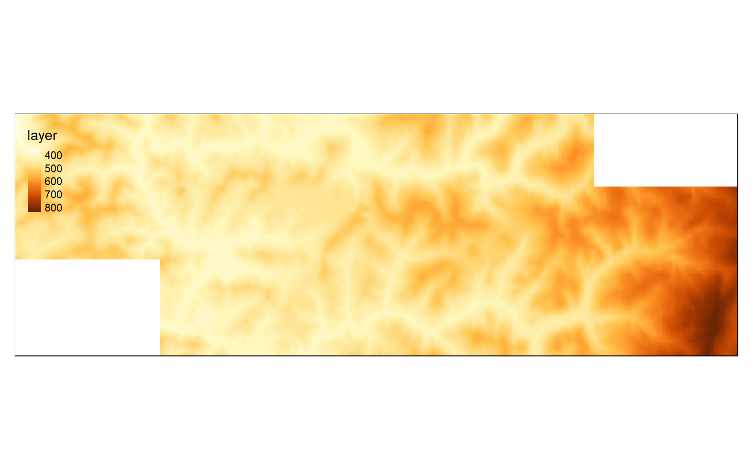
In all the results above the data have filled a rectangular extent. What if you would like to extract values that fall within an irregular extent as defined by a raster mask or vector polygon layer? This can be accomplished using the mask() function. In the example, I have extracted out cells that occur within the watershed boundaries only. Note that the raster grid is still rectangular, or there is a complete set of rows and columns. However, cells outside the mask have been coded to a NA, Null, or NoDATA assignment. Regardless of the shape of the area of interest, all raster grids must be rectangular.
elev_mask <- mask(elev, ws)
tm_shape(elev_mask)+
tm_raster(style= "cont")+
tm_shape(ws)+
tm_borders(col="black")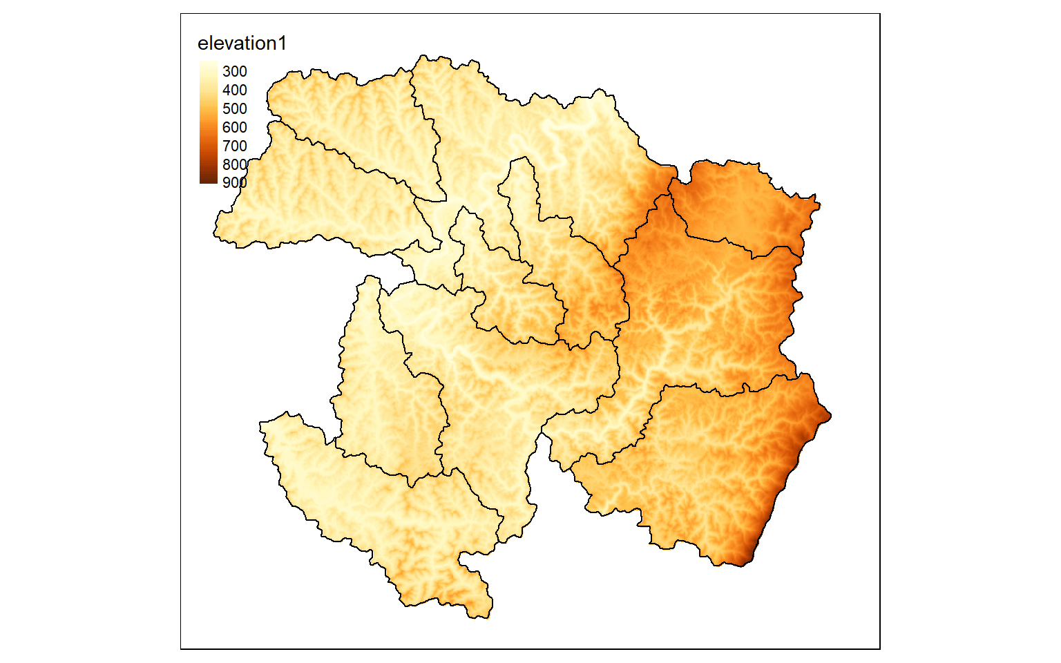
Resample and Aggregate
It is also possible to change the cell size of a grid. The raster package provides three different functions to accomplish this.
- resample(): change cell size using bilinear interpolation (inverse distance weighted average of nearest 4 cell values) or nearest neighbor (only considers nearest cell value)
- aggregate(): increase the cell size by a defined factor and calculate a statistic from the smaller, original cells to populate the larger, new cells
- disaggregate(): make cell size smaller by a defined factor
When resampling raster grids, make sure to use a method appropriate for the input raster data type. For example, taking the average or using bilinear interpolation would not be appropriate for a categorical grid since you can’t average categories. Instead, you would want to use maximum, minimum, or majority. Nearest neighbor is also appropriate for categorical data since no averaging is applied.
In the example, I have used the aggregate() function to increase the cell size by a factor of 5. So, the 30 m grid is converted to a 150 m grid. The new cells will be populated with the mean from the original cells that fall within them. The cell size can be checked by calling the resulting object.
elev_agg <- aggregate(elev, fact=5, fun=mean)
elev_agg
class : RasterLayer
dimensions : 385, 423, 162855 (nrow, ncol, ncell)
resolution : 150, 150 (x, y)
extent : 551467.6, 614917.6, 4335125, 4392875 (xmin, xmax, ymin, ymax)
crs : +proj=utm +zone=17 +datum=WGS84 +units=m +no_defs
source : memory
names : elevation1
values : 242, 955.2 (min, max)
tm_shape(elev_agg)+
tm_raster(style= "cont")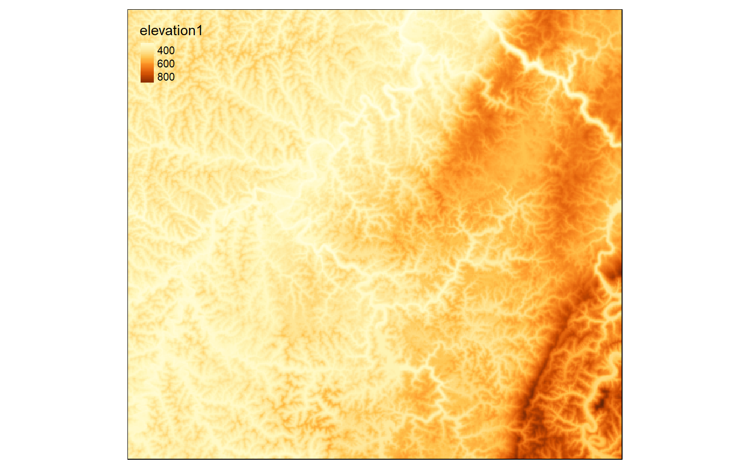
Reclassify
Reclassify is used to change or recode cell values in a grid. When reclassifying a continuous grid, a range of values will be recoded or binned to a new value. So, the result of reclassify is always a categorical raster grid.
Before reclassifying a grid, you must generate a matrix of values to define the reclassification. In the example, I am generating a matrix with four rows and three columns. I first create a vector of values then convert them to a matrix using the matrix() function. Here is a description of the reclassification being performed.
- 0 > value <= 300: 1
- 300 > value <= 500: 2
- 500 > value <= 800: 3
- 800 > value <= 10,000: 4
Note that these ranges have no gaps. Also, I generally set the smallest and largest values to be much smaller or larger than the values in the grid to make sure all values are included.
In the reclassify() function I provide the raster data to be reclassified (elev), the matrix used to describe the reclassification (m), and the right argument. When right is set to TRUE, the right side of each class will be closed. So, the largest value is included in that bin as opposed to the next bin. For example, 300 would be coded as 1 as opposed to 2 in the example.
m <- c(0, 300, 1, 300, 500, 2, 500,
800, 3, 800, 10000, 4)
m <- matrix(m, ncol=3, byrow = TRUE)
dem_re <- reclassify(elev, m, right=TRUE)
tm_shape(dem_re)+
tm_raster(style= "cat")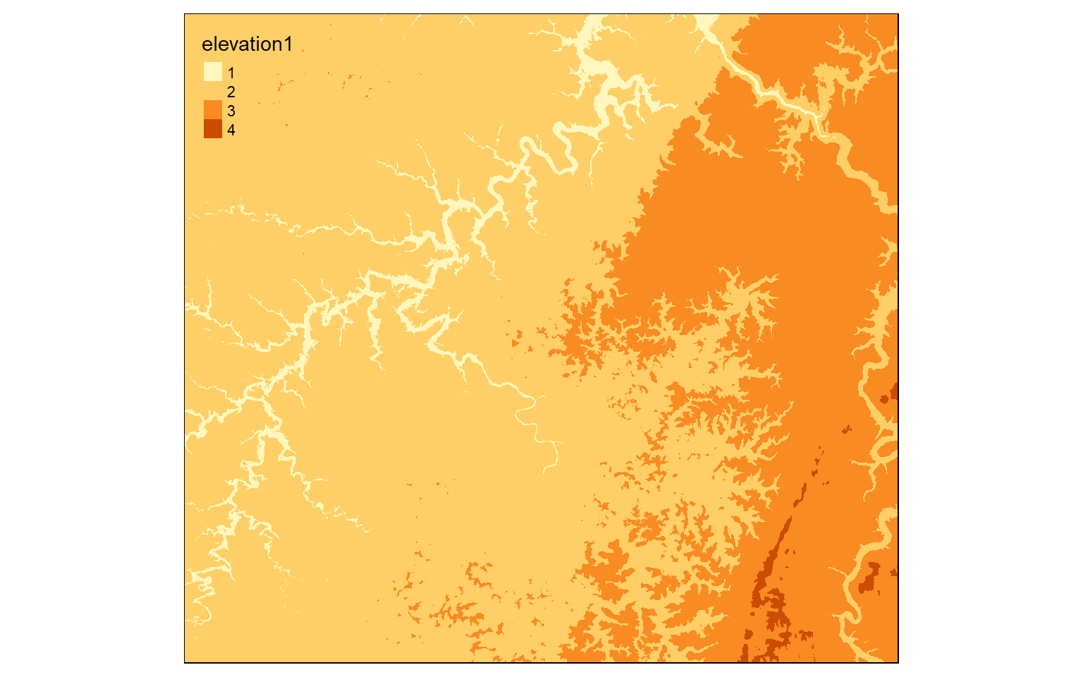
Now, I am reclassifying the land cover, a categorical raster grid, to “Not Forest” and “Forest”. All forest types have codes between 40 and 50 (41, 42, and 43). So, that range is coded to 1 and all other ranges are coded to 0.
m2 <- c(10, 40, 0, 40, 50, 1, 50, 100, 0)
m2 <- matrix(m2, ncol=3, byrow = TRUE)
lc_re <- reclassify(lc, m2, right=TRUE)
tm_shape(lc_re)+
tm_raster(style= "cat", labels = c("Not Forest", "Forest"), palette = c("gray", "darkolivegreen"))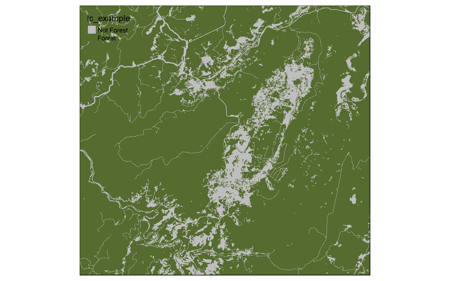
Raster Math
Performing mathematical operations on grids is easy in R. The syntax is the same as operations applied to vectors or matrices. In the first example, the elevation grid is being multiplied by a conversion factor to convert the units from meters to feet. This operation will be applied to each cell and the result will be returned to a new cell in the output.
elev_ft <- elev*3.28084
tm_shape(elev_ft)+
tm_raster(style= "cont")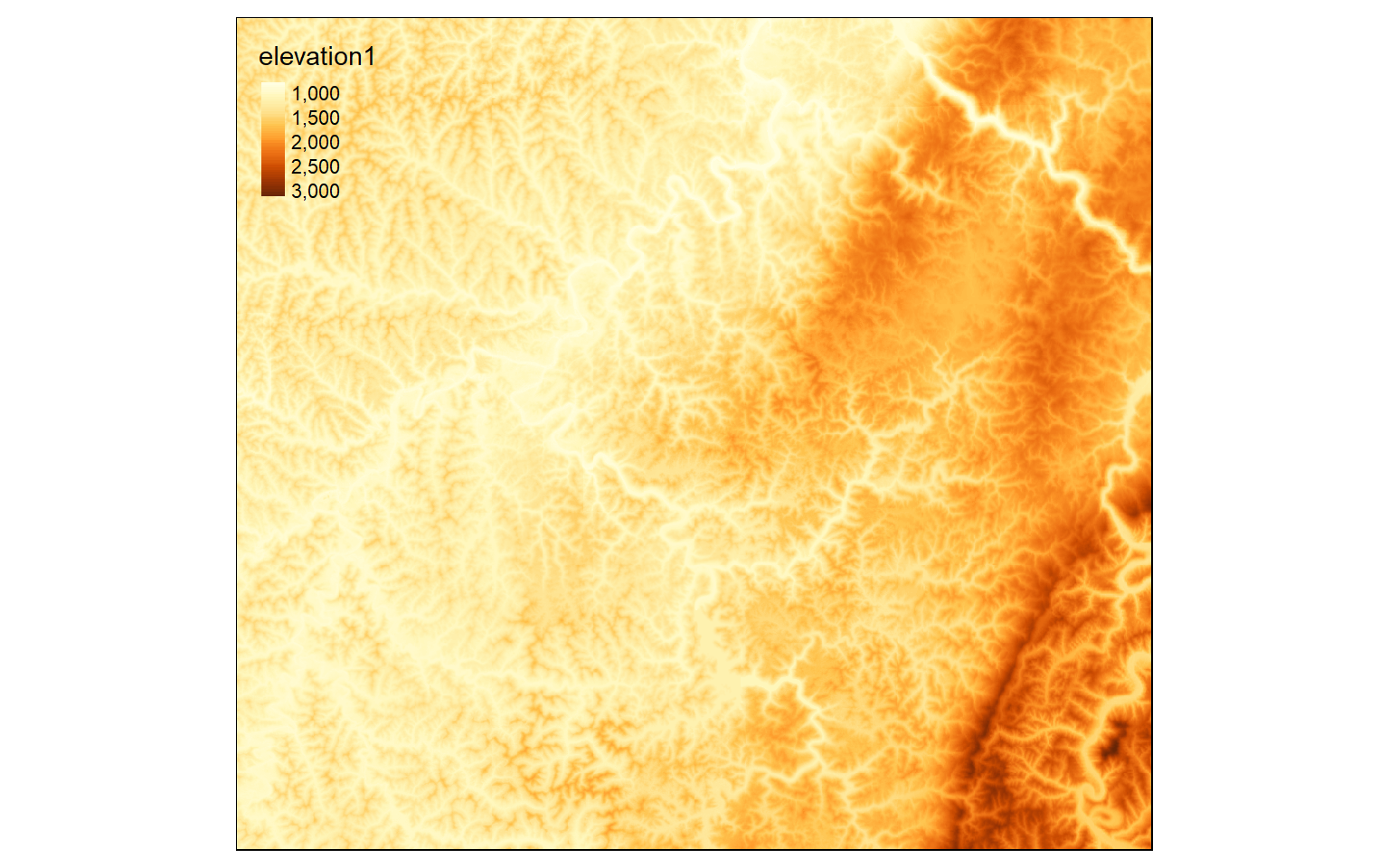
In this example, I am dividing the elevation grid in feet by the elevation grid in meters. This returns the conversion factor at each cell location.
conversion <- elev_ft/elev
tm_shape(conversion)+
tm_raster(style= "cont")
When Boolean operations are applied to raster grids, the result will be 0 or 1. 0 always indicates that the logic evaluated to FALSE while 1 indicates TRUE. In the example below, I am trying to find all cells that have an elevation greater than 600 meters. Those that do are coded to 1 while those that don’t are coded to 0. TRUE areas are shown in red.
elev_600 <- elev > 600
tm_shape(elev_600)+
tm_raster(style= "cat", labels = c("No", "Yes"), palette = c("gray", "darkred"))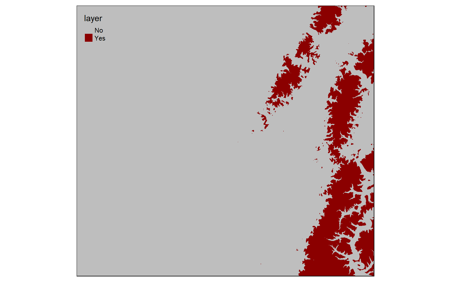 In this example, I am finding all cells coded to 0 or FALSE from the prior example. This effectively inverts the result: now cells that are less than or equal to 600 meters in elevation are coded to TRUE while high elevation cells are coded to FALSE.
We will explore these methods in more detail below in the context of conservative models.
invert <- elev_600 == 0
tm_shape(invert)+
tm_raster(style= "cat", labels = c("No", "Yes"), palette = c("gray", "darkred"))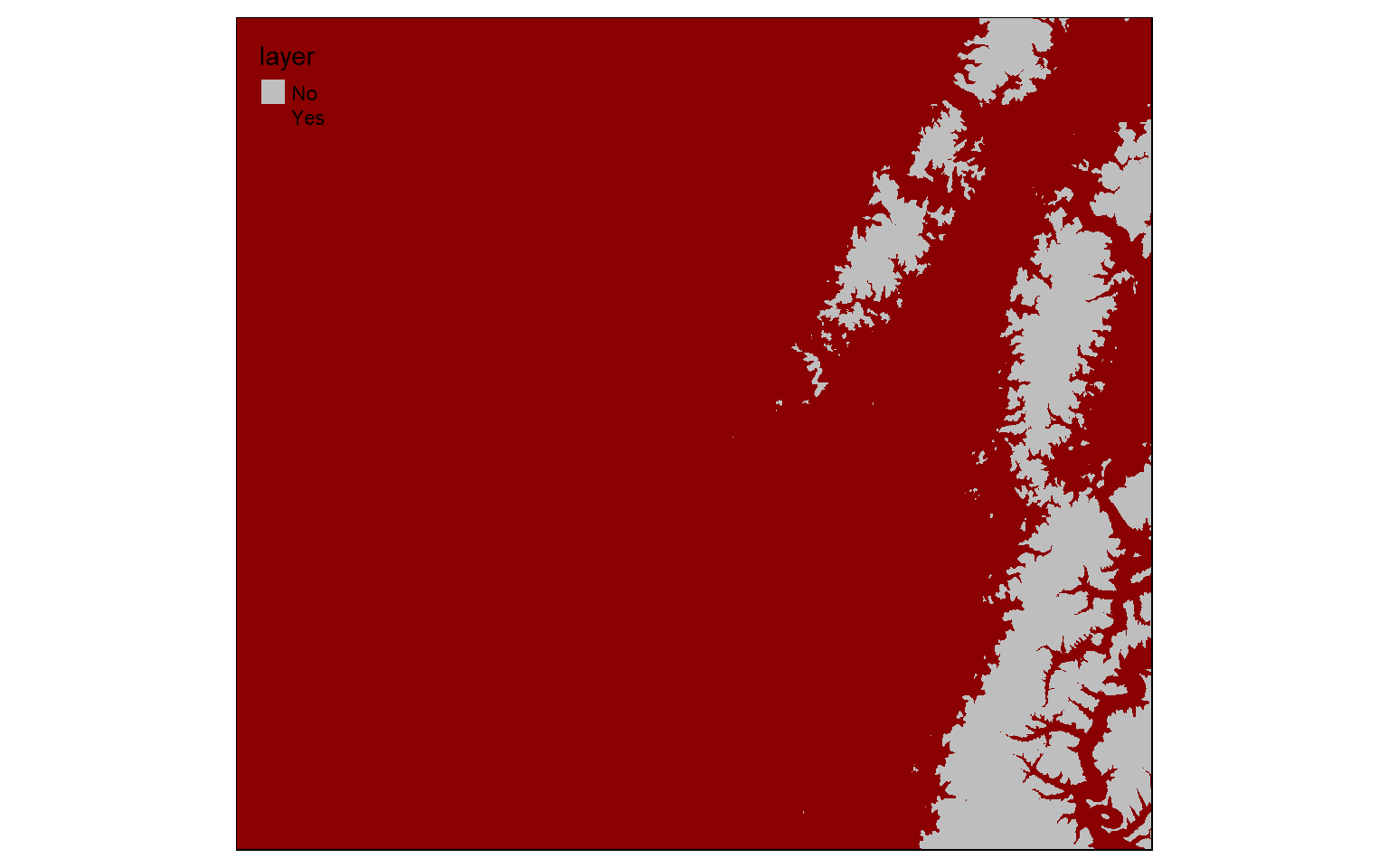
Raster Summarization
It is possible to extract cell values at point locations. This is often used to generate sample data for analyses and machine learning where training data are required.
The extract() function can accomplish this task. In the first example, I am extracting the elevation values at random points. the sp argument is used to specify whether spatial information should be included in the output. When defined as TRUE, spatial information will be maintained and the result will be a SpatialPointsDataFrame. I am also using the st_as_sf() function to convert the sp object to an sf object.
pnt_elev <- st_as_sf(raster::extract(elev, pnts, sp=TRUE))Now, I am visualizing the results by plotting the extracted elevation to the point feature size aesthetic.
tm_shape(elev)+
tm_raster(style= "cont")+
tm_shape(pnt_elev)+
tm_bubbles(size="elevation1")+
tm_layout(legend.outside=TRUE)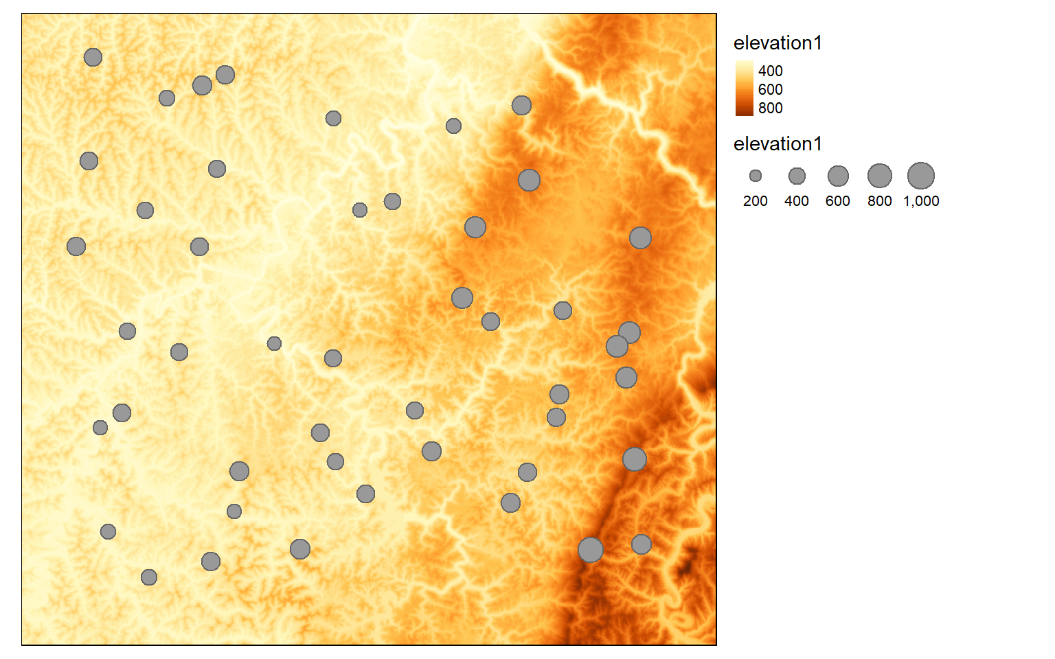
It is also possible to summarize raster data relative to areas or polygons. Since now there can be multiple cells within the areas, you must indicate a statistical measure to return. Here, I am extracting the mean elevation by watershed. I then map the results. Depending on the spatial resolution of the grid and the number and complexity of the polygons, these calculations can take some time.
ws_mn_elev <- st_as_sf(raster::extract(elev, ws, fun=mean, sp=TRUE))tm_shape(ws_mn_elev)+
tm_polygons(col="elevation1")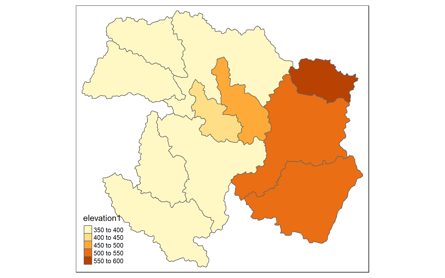
Distance and Density grids
Euclidean distance is simply a measure of the straight line distance from a cell to a source feature. In the first example, I am calculating the distance from each cell to the nearest point feature. To start, I generate a blank grid by making a copy of the elev data then converting all cell values to NA. I then use the distanceFromPoints() function to repopulate the grid with the distance measurement. This function requires an sp object, so I make the conversion within the function. The resulting distance will be in the map units, in this case meters. You can convert to different units using raster math.
blank <- elev
blank[] <- NA

dist <- distanceFromPoints(blank, as(pnts, "Spatial"))

tm_shape(dist)+
tm_raster(style= "cont")+
tm_shape(pnts)+
tm_bubbles()+
tm_layout(legend.outside=TRUE)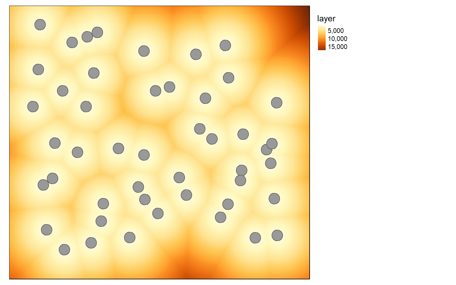
When calculating distance from line features, you must first convert the vector data to a raster grid. I begin by creating a blank grid then populating it with 1 at locations where there is an interstate using the rasterize() function. I then convert the cells to points using rasterToPoints(). I can then use the distanceFromPoints() function to generate the distance surface. Note that this process can be slow.
blank <- elev
blank[] <- NA

interstates$CLASS <- as.factor(interstates$CLASS)
interstate.r <- rasterize(interstates, blank, "CLASS")

interstate_points <- rasterToPoints(interstate.r, spatial=TRUE)

interstate.d <- distanceFromPoints(blank, interstate_points)

tm_shape(interstate.d)+
tm_raster(style= "cont")+
tm_shape(interstates)+
tm_lines(col="black")+
tm_layout(legend.outside = TRUE)
Kernel density surfaces can be created using the sp.kde() function from the spatialEco() package. This function will not accept sf objects, so it is necessary to convert the point data to sp. The search radius must be provided in the map units using the bw, or bandwidth, argument. I am using a value of 500 meters in this example. Larger values will result in a more generalized pattern. There is not necessarily a correct radius, as this depends on whether you are interested in local patterns or more generalized patterns. The blank grid created above is being used to determine the extent and cell size of the result. This process can be slow if a large number of point features is included, a large spatial extent is calculated, and/or a small cell size is used.
blank <- elev

str_sp <- as(str, Class="Spatial")

str_den <- sp.kde(x=str_sp, bw=500, newdata=blank)tm_shape(str_den)+
tm_raster(style= "cont")+
tm_layout(legend.outside = TRUE)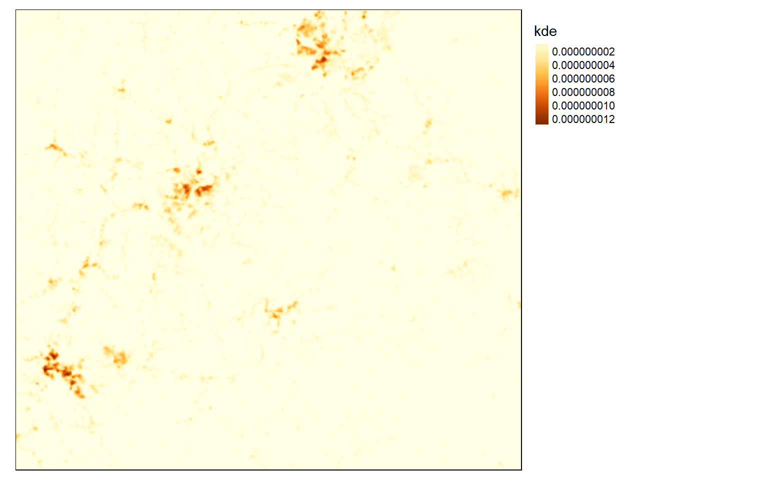
Conservative Models
Conservative models yield a TRUE/FALSE or binary output. A site or cell either meets the criteria or it does not. You can use the methods discussed above to produced conservative models by generating binary surfaces for each criterion then multiplying them together to obtain a final model.
In this example, we are trying to determine locations that are suitable for a new hotel. The location should be:
- At an elevation above 500 meters
- On a slope less than 15 degrees
- Not further than 3 km from an airport
- Not further than 5 km from an interstate
To begin, I first visualize the input vector and raster data.
tm_shape(elev)+
tm_raster(style= "cont")+
tm_shape(airports)+
tm_bubbles(col="black")+
tm_shape(interstates)+
tm_lines()+
tm_layout(legend.outside = TRUE)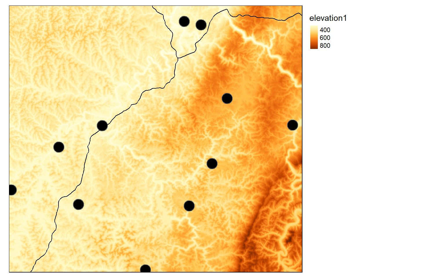
Next, I create Euclidean distance grids for distance from airports and distance from interstates using the methods demonstrated above.
blank <- elev
blank[] <- NA

airport.d <- distanceFromPoints(blank, as(airports, "Spatial"))

tm_shape(airport.d)+
tm_raster(style= "cont")+
tm_shape(airports)+
tm_bubbles(col="black")+
tm_layout(legend.outside = TRUE)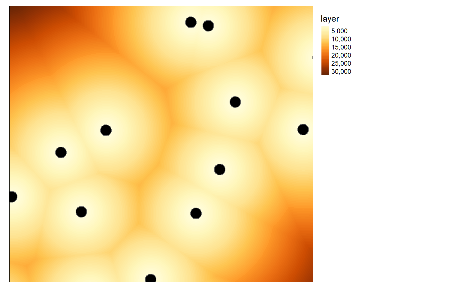
blank <- elev
blank[] <- NA

interstate.r <- rasterize(interstates, blank, "CLASS")

interstate_points <- rasterToPoints(interstate.r, spatial=TRUE)

interstate.d <- distanceFromPoints(blank, interstate_points)

tm_shape(interstate.d)+
tm_raster(style= "cont")+
tm_shape(interstates)+
tm_lines(col="black")+
tm_layout(legend.outside = TRUE)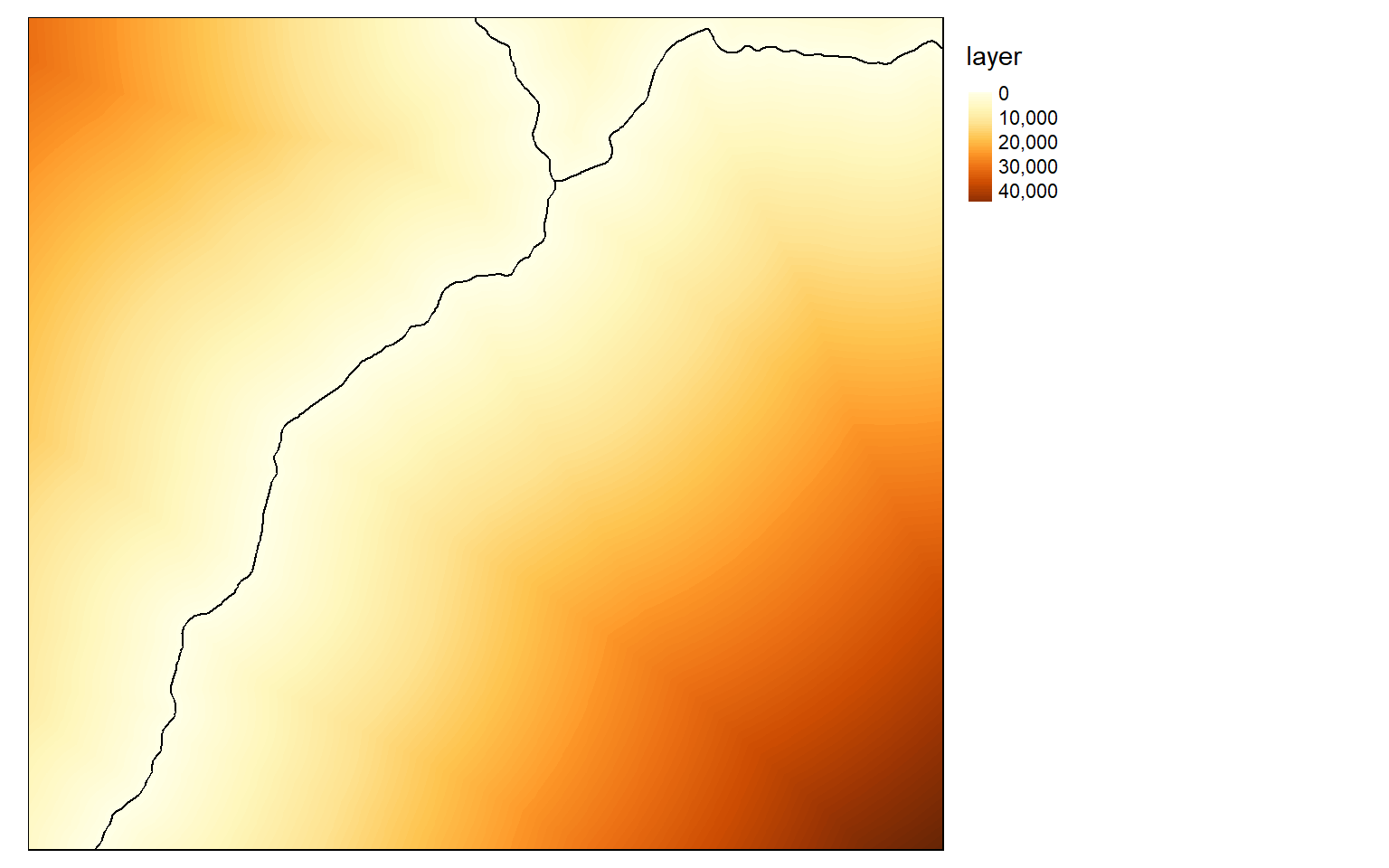
I now have the four required input raster grids. The next step is to obtain binary surfaces for each criterion. This can be accomplished using logical operators and raster math.
#Create Binary Surfaces
#Elevation > 500
#Slope < 15
#Airports < 3000
#Interstates < 5000

elev_binary <- elev > 500
ele_b <- tm_shape(elev_binary)+
tm_raster(style="cat")+
tm_layout(main.title="Elevation")

slp_binary <- slp < 15
slp_b <- tm_shape(slp_binary)+
tm_raster(style="cat")+
tm_layout(main.title="Slope")

air_binary <- airport.d < 7000
airport_b <- tm_shape(air_binary)+
tm_raster(style="cat")+
tm_layout(main.title="Airports")

inter_binary <- interstate.d < 5000
interstate_b <- tm_shape(inter_binary)+
tm_raster(style="cat")+
tm_layout(main.title="Interstates")

tmap_arrange(ele_b, slp_b, airport_b, interstate_b)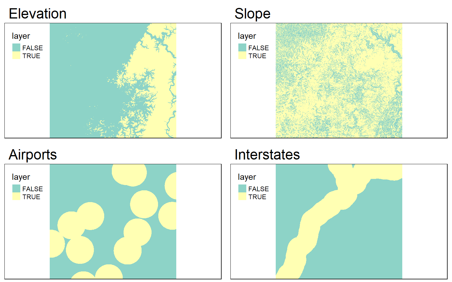
Once the binary surfaces have been generated, I simply multiply them together to obtain a final suitability model. A location or cell would have to be TRUE (or 1) for all criteria in order for 1 to be returned.
Based on the required conditions, few cells in the extent meet all the criteria.
c_model <- elev_binary*slp_binary*air_binary*inter_binary

tm_shape(c_model)+
tm_raster(style="cat")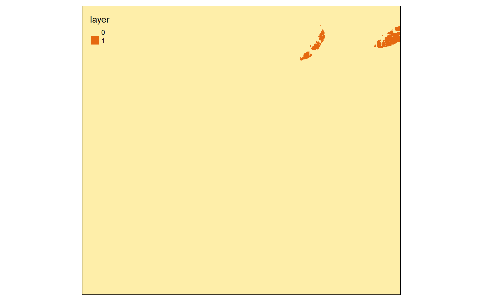
Liberal Models
What if you wanted more “gray levels” or a range of suitability scores in the output as opposed to only yes or no? This could be accomplished using weighted overlay. The goal here is to combine scored grids and weights to obtain a model with a range of suitability values. Let’s repeat the process above relating to determining a location for a hotel using liberal modeling methods. Here are the criteria:
- High elevation preferred
- Shallow slope preferred
- Close to airports preferred
- Close to interstates preferred
I will not recalculate the distance grids, as I already have them from the conservative modeling process completed above.
All scores should be on the same scale, so I will rescale the data from 0 to 1 using the range of values in each grid. The minimum and maximum values from the grids can be extracted using the cellStats() function. I then use raster math to scale each grid from 0 to 1. For all surfaces except elevation, I am subtracting from 1 since low values are preferred.
#Rescale from 0-1
#High elevation is good
#Low slope is good
#Close to airports is good
#Close to interstates is good

elev_min <- cellStats(elev, stat=min)
elev_max <- cellStats(elev, stat=max)
elev_score <- ((elev - elev_min)/(elev_max - elev_min))
ele_s <- tm_shape(elev_score)+
tm_raster(style="cont")+
tm_layout(main.title="Elevation")

slp_min <- cellStats(slp, stat=min)
slp_max <- cellStats(slp, stat=max)
slp_score <- 1 - ((slp - slp_min)/(slp_max - slp_min))
slp_s <- tm_shape(slp_score)+
tm_raster(style="cont")+
tm_layout(main.title="Slope")

air_min <- cellStats(airport.d, stat=min)
air_max <- cellStats(airport.d, stat=max)
air_score <- 1 - ((airport.d - air_min)/(air_max - air_min))
airport_s <- tm_shape(air_score)+
tm_raster(style="cont")+
tm_layout(main.title="Airports")

inter_min <- cellStats(interstate.d, stat=min)
inter_max <- cellStats(interstate.d, stat=max)
inter_score <- 1- (interstate.d - inter_min)/(inter_max - inter_min)
interstate_s <- tm_shape(inter_score)+
tm_raster(style="cont")+
tm_layout(main.title="Interstates")

tmap_arrange(ele_s, slp_s, airport_s, interstate_s)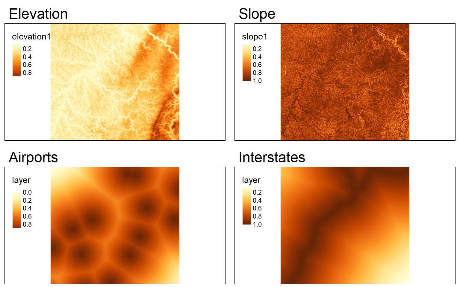
Once each criterion has been converted to the same scale and scored, then I multiply them together to obtain a model. It is also possible to incorporate weights if the criteria are of different importance.
This will create a final suitability model that takes into account each criterion and its relative importance. In contrast to a conservative model, a range of suitability scores will be returned.
#Weight for elevation = 0.1
#Weight for slope =0.4
#Weight for Airport Distance = 0.2
#Weight for Interstate Distance =0.3

wo_model <- (elev_score*.1)+(slp_score*.4)+(air_score*.2)+(inter_score*.3)

tm_shape(wo_model)+
tm_raster(style="cont")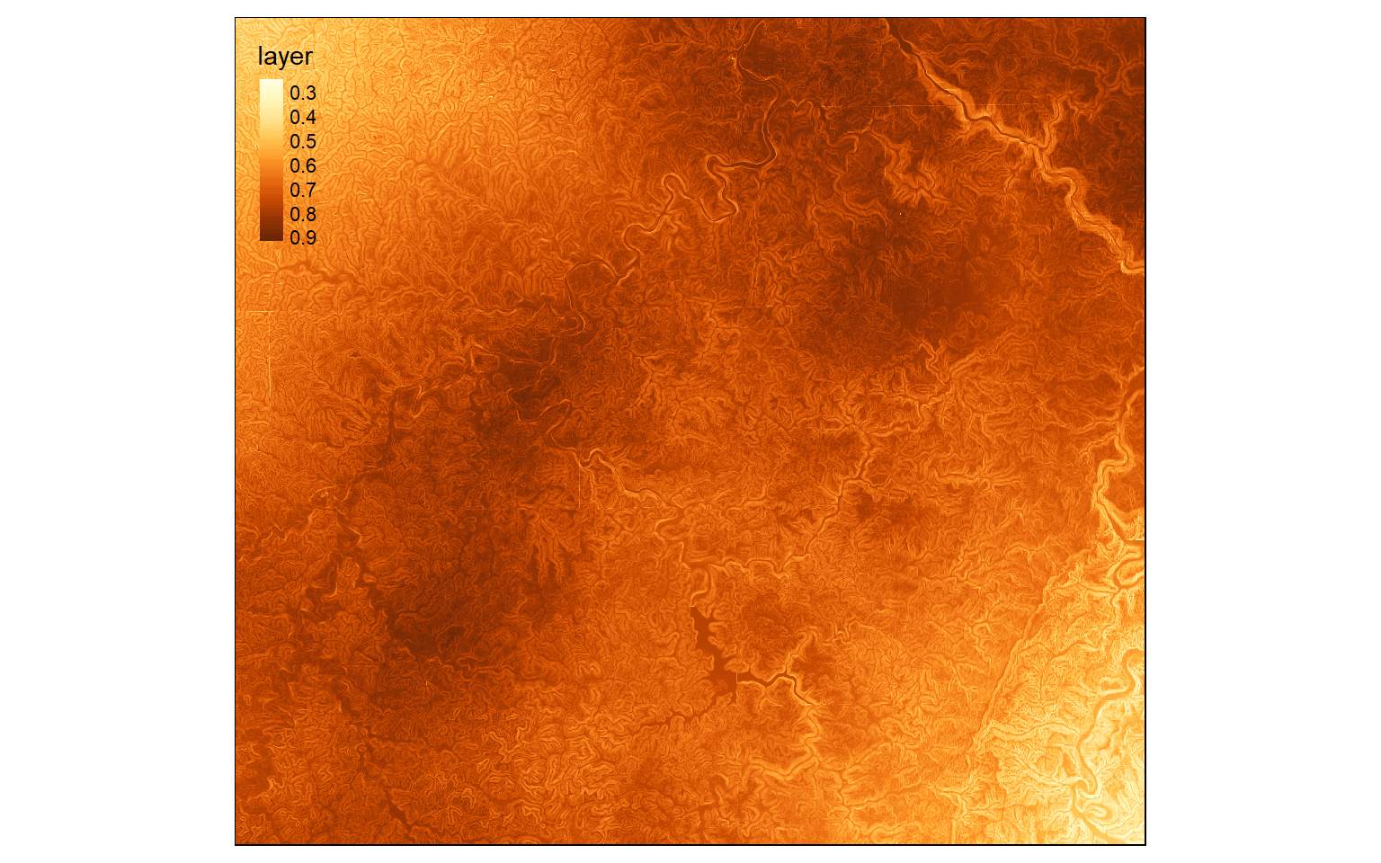
Lastly, reclassification can be used to define suitability ranges based on cut-off values as demonstrated below.
m3 <- c(0, .5, 0, .5, .6, 1, .6, 1, 2)
m3 <- matrix(m3, ncol=3, byrow = T)

wo_model_re <- reclassify(wo_model, m3, right=T)

tm_shape(wo_model_re)+
tm_raster(style= "cat", labels = c("Not Suitable", "Suitable", "Very Suitable"),
palette = c("gray", "yellow", "red"),
title="Weight Oberlay Model")+
tm_layout(legend.outside = TRUE)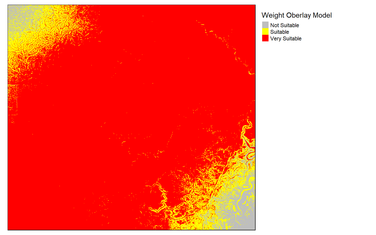
Concluding Remarks
In this section, I have tried to focus on techniques that I commonly use when working with and analyzing raster data. Again, you will likely need to solve different types of problems to analyze your own data. The documentation for the raster package is very thorough, so it is a great resource, and there are a variety of additional resources on the web.
We will work with raster data in later sections when we make models using machine learning, so you will get more practice working with and manipulating these data in R.
Before we move on to machine learning-based modeling, we will explore the new terra package and working with LiDAR point cloud data and remotely sensed imagery in R in the following sections.