Vector-Based Spatial Analysis in R

Objectives

Use the sf package to read in and prepare vector data
Filter rows, select columns, and randomly sample data using dplyr
Summarize attributes and compare groups
Join tables and perform table calculations
Perform a variety of geoprocessing tasks including dissolve, clip, intersect, union, erase, and symmetrical difference
Summarize point, line, and polygon data relative to polygons
Simplify geometries
Create tessellations

Overview

In this section we will explore a wide variety of techniques for working with and analyzing vector geospatial data in R. Specifically, we will focus on methods made available in the sf package. There are additional libraries for reading in and working with vector geospatial data in R, such as sp. However, I prefer sf. If you work at all with PostgreSQL and PostGIS you will observe lots of similarities. For example, functions designed to work on spatial data in sf and PostGIS are all prefixed with “st_”. Also, they both make use of an object-based vector data model where the geometry and attributes are stored in the same table.

You will need to load in the following packages to execute the provided examples. We will use tmap to visualize the results of our analyses.

library(tmap)
library(tmaptools)
library(rgdal)
library(sf)
library(dplyr)
library(ggplot2)
library(tidyr)

We will use a variety of data layers in this module. I have provided a description of the layers below. The link at the bottom of the page provides the example data and R Markdown file used to generate this module.

circle.shp: a circle (shapefile)
Triangles.shp: a triangle (shapefile)
extent.shp: bounding box extent of circle and triangle (shapefile)
interstates.shp: interstates in West Virginia as lines (shapefile)
rivers.shp: major rivers in West Virginia as lines (shapefile)
towns.shp: point features of large towns in West Virginia (shapefile)
wv_counties.shp: West Virginia county boundaries as polygons (shapefile)
harvest.csv: CSV table of deer harvest data by county from the West Virginia Division of Natural Resources (WVDNR) (shapefile)
tornadoes: point features of tornadoes across US (feature class)
cities: point features of cities in the US (feature class)
interstates:interstates in US as lines (feature class)
Us_eco_ref_l3: ecological regions of the US as polygons (feature class)
states: US state boundaries (feature class)

All vector files are read in using the st_read() function from sf. This will generate a data frame with a column for each attribute and an additional column to store the geographic information. The table is loaded using read.csv() from base R.

circle <- st_read("vector_analysis/shapes/circle.shp")
triangle <- st_read("vector_analysis/shapes/triangle.shp")
ext <- st_read("vector_analysis/shapes/extent.shp")
inter <- st_read("vector_analysis/wv/interstates.shp")
rivers <- st_read("vector_analysis/wv/rivers.shp")
towns <- st_read("vector_analysis/wv/towns.shp")
wv_counties <- st_read("vector_analysis/wv/wv_counties.shp")
harvest <- read.csv("vector_analysis/wv/harvest.csv", sep=",", header=TRUE, stringsAsFactors=TRUE)
torn <- st_read(dsn="vector_analysis/us.gdb", "tornadoes")
us_cities <- st_read(dsn="vector_analysis/us.gdb", "cities")
us_inter <- st_read(dsn="vector_analysis/us.gdb", "interstates")
eco <- st_read(dsn="vector_analysis/us.gdb", "us_eco_ref_l3")
states <- st_read(dsn="vector_analysis/us.gdb", "states")

Data Summarization and Querying

Let’s start by mapping the ecological region boundaries using tmap. I am using color to show the Level 1 ecoregion name as a qualitative variable. I am also plotting the legend outside of the map space.

tm_shape(eco)+
tm_polygons(col="NA_L1NAME")+
tm_layout(legend.outside=TRUE)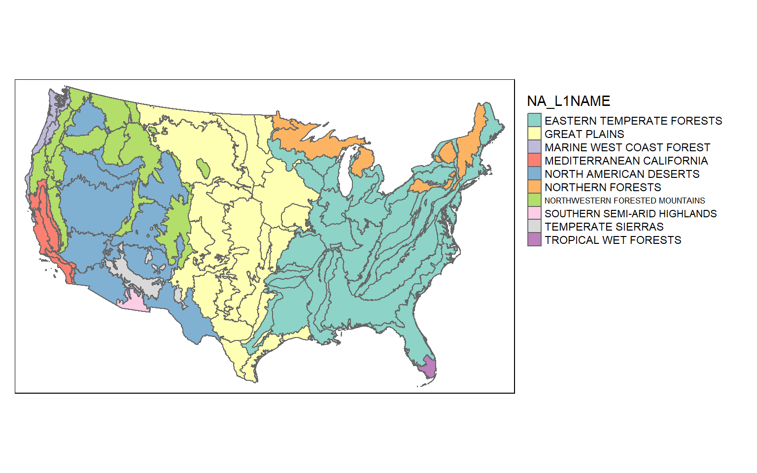

Since sf objects are data frames, we can work with and manipulate them using a variety of functions that accept data frames. In the next code block I am using dplyr to count the number of polygons belonging to each Level 1 ecoregion. The result is a tibble. You can see that the eastern temperate forest has the largest number of polygons associated with it.

This process is the same as working with any data frame. This is one of the benefits of using sf to read vector data into R.

eco_l1_names <- eco %>% group_by(NA_L1NAME) %>% count()
print(eco_l1_names)
Simple feature collection with 10 features and 2 fields
Geometry type: MULTIPOLYGON
Dimension:     XY
Bounding box:  xmin: -2356069 ymin: -1334738 xmax: 2258225 ymax: 1565791
Projected CRS: USA_Contiguous_Albers_Equal_Area_Conic
# A tibble: 10 x 3
   NA_L1NAME                           n                                   Shape
 * <chr>                           <int>                      <MULTIPOLYGON [m]>
 1 EASTERN TEMPERATE FORESTS         890 (((12584.16 -822638.3, 12354.51 -82255~
 2 GREAT PLAINS                       46 (((-769984.9 251560.7, -770080.1 25176~
 3 MARINE WEST COAST FOREST           75 (((-2333217 365413.2, -2333228 365412.~
 4 MEDITERRANEAN CALIFORNIA           40 (((-2274246 355038.8, -2274243 355037,~
 5 NORTH AMERICAN DESERTS             13 (((-1942206 114548.6, -1942367 114489,~
 6 NORTHERN FORESTS                   43 (((39799.58 1144755, 39725.01 1145150,~
 7 NORTHWESTERN FORESTED MOUNTAINS    38 (((-2145392 540135.2, -2145403 540106,~
 8 SOUTHERN SEMI-ARID HIGHLANDS        2 (((-1347590 -385879.1, -1347294 -38584~
 9 TEMPERATE SIERRAS                  11 (((-1461916 -17363.68, -1461708 -17625~
10 TROPICAL WET FORESTS               92 (((1416141 -1332814, 1416433 -1332827,~

Records, rows, or geospatial features can be extracted using the filter() function from dplyr. In the next code block I am extracting out all features that are within the great plains Level 1 ecoregion. I then map the extracted features and use color to differentiate the Level 2 ecoregions. Note that I use droplevels() here to remove any Level 2 names that are not in the extracted Level 1 ecoregion. This is common practice when subsetting factors, as you might remember.

eco_gp <- eco %>% filter(NA_L1NAME=="GREAT PLAINS")
eco_gp$NA_L2NAME <- as.factor(eco_gp$NA_L2NAME)
eco_gp$NA_L2NAME <- droplevels(eco_gp$NA_L2NAME)
tm_shape(eco_gp)+
tm_polygons(col="NA_L2NAME")+
tm_layout(legend.outside=TRUE)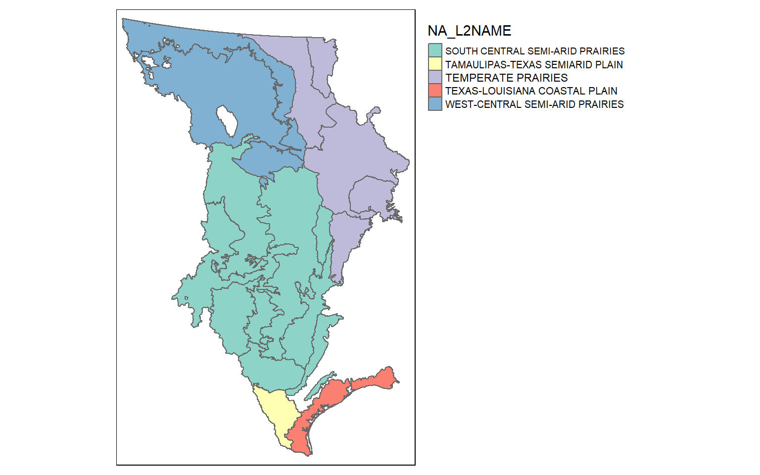

Again, since sf objects are just data frames you can explore the tabulated data using a variety of functions and methods. As an example, I am using ggplot2 to compare county-level population by sub-region of the US. Since the geographic information is not needed here, it is simply ignored.

ggplot(states, aes(x=as.factor(SUB_REGION), y=POP2000, fill=as.factor(SUB_REGION)))+
geom_boxplot()

As a similar example, I am using dplyr to obtain the mean county population for each sub-region. Note that the geometry data are automatically included even though we did not specify this. The results are stored as a tibble.

sub_summary <- states %>% group_by(SUB_REGION) %>% summarize(mn_pop = mean(POP2000))
print(sub_summary)
Simple feature collection with 9 features and 2 fields
Geometry type: GEOMETRY
Dimension:     XY
Bounding box:  xmin: -2354936 ymin: -1294964 xmax: 2256319 ymax: 1558806
Projected CRS: USA_Contiguous_Albers_Equal_Area_Conic
# A tibble: 9 x 3
  SUB_REGION    mn_pop                                                     Shape
  <chr>          <dbl>                                            <GEOMETRY [m]>
1 E N Cen     9031007. MULTIPOLYGON (((533953.8 1186943, 525298.4 1174178, 5171~
2 E S Cen     4255702. POLYGON ((722689.3 -772545, 711350.8 -767348.4, 701587.7~
3 Mid Atl    13223954. MULTIPOLYGON (((1487830 387523.5, 1451677 380757.5, 1442~
4 Mtn         2271537. POLYGON ((-2030398 415961.6, -2037196 426027.7, -2035245~
5 N Eng       2320420. MULTIPOLYGON (((1829205 817426.1, 1826757 828696.4, 1818~
6 Pacific    14395723. MULTIPOLYGON (((-2294824 877285.2, -2290551 897464.2, -2~
7 S Atl       5752129. MULTIPOLYGON (((906637.8 -748539.9, 886874.5 -749470.2, ~
8 W N Cen     2748248. POLYGON ((18888.98 -56220.13, 3706.183 -56019.98, -533.3~
9 W S Cen     7861212. MULTIPOLYGON (((-991765.9 -583758, -998446.9 -579477.8, ~

Each tornado point has a Fujita scale attribute, a measure of tornado intensity. In this example I am counting the number of tornadoes by Fujita category. As expected, severe tornadoes occur much less frequently. Note again that the geometric information is automatically added to the result.

torn_f <- torn %>% group_by(F_SCALE) %>% count()
print(torn_f)
Simple feature collection with 6 features and 2 fields
Geometry type: GEOMETRY
Dimension:     XY
Bounding box:  xmin: -2229714 ymin: -1311837 xmax: 2086534 ymax: 1418053
Projected CRS: USA_Contiguous_Albers_Equal_Area_Conic
# A tibble: 6 x 3
  F_SCALE     n                                                            Shape
*   <int> <int>                                                   <GEOMETRY [m]>
1       0  1236 MULTIPOINT ((-2229714 246118.9), (-2199342 -36882.5), (-2168475~
2       1   531 MULTIPOINT ((-2159739 302537.5), (-1822649 1159463), (-1422559 ~
3       2   168 MULTIPOINT ((-1615053 1032388), (-688980.6 -448566.8), (-653282~
4       3    58 MULTIPOINT ((-529000.4 119032.7), (-445209.2 -234840.9), (-4320~
5       4     6 MULTIPOINT ((78006.03 85549.83), (324747.5 247499.7), (537752.1~
6       5     1                                       POINT (-301565.4 18923.11)

In this example, I am extracting all tornadoes that have a Fujita value larger than or equal to 3 using dplyr. I then plot them as points using tmap.

torn_hf <- torn %>% filter(F_SCALE >= 3)

tm_shape(states)+
tm_polygons(col="tan")+
tm_shape(torn_hf)+
tm_bubbles(col="red")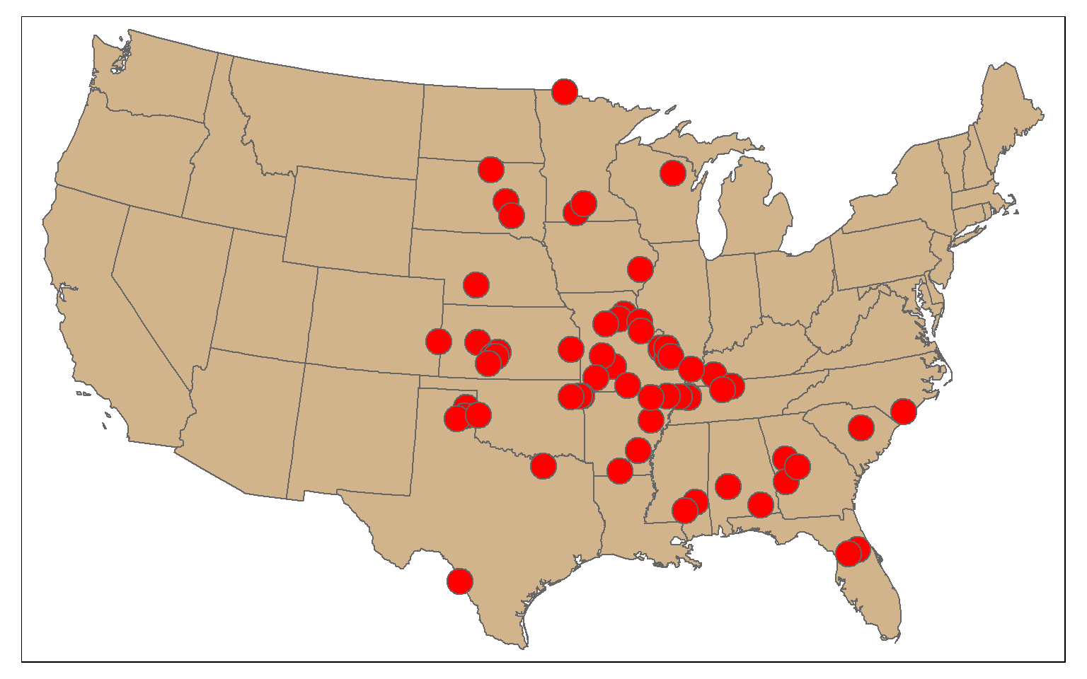

It is also possible to subset columns or attributes using the select() function from dplyr. Using this method, I extract out only the state name, sub-region, and population attributes using the code below. Note again that the geometric information is automatically included.

states_sel <- states %>% dplyr::select(STATE_NAME, SUB_REGION, POP2000)
glimpse(states_sel)

Table Joins

Tabulated data can be joined to spatial features if they share a common field. This is known as a table join. In the example, I am joining the deer harvest data to the counties. First, I change the second column’s name to “NAME” as opposed to “COUNTY” so that the column name matches that of the polygon features. I then use left_join() from dplyr to associate the data using the common “NAME” field.

I then map the total number of deer harvested by county.

names(harvest)[2] <- "NAME"
counties_harvest <- inner_join(wv_counties, harvest, by="NAME")

tm_shape(counties_harvest) +
tm_polygons(col="TOTALDEER", title = "Harvest")+
tm_compass()+
tm_scale_bar()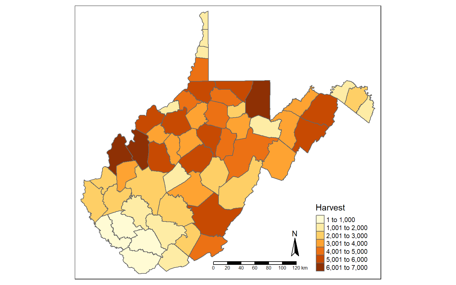

New attribute columns can be generated using the mutate() function from dplyr. Using this function, I calculate the density of deer harvest as deer per square mile using the “TOTALDEER” and “SQUARE_MIL” fields. The density is then written to a new column called “DEN”.

counties_harvest <- mutate(counties_harvest, DEN = TOTALDEER/SQUARE_MIL)

tm_shape(counties_harvest)+
tm_polygons(col="DEN", title = "Harvest Density")+
tm_compass()+
tm_scale_bar()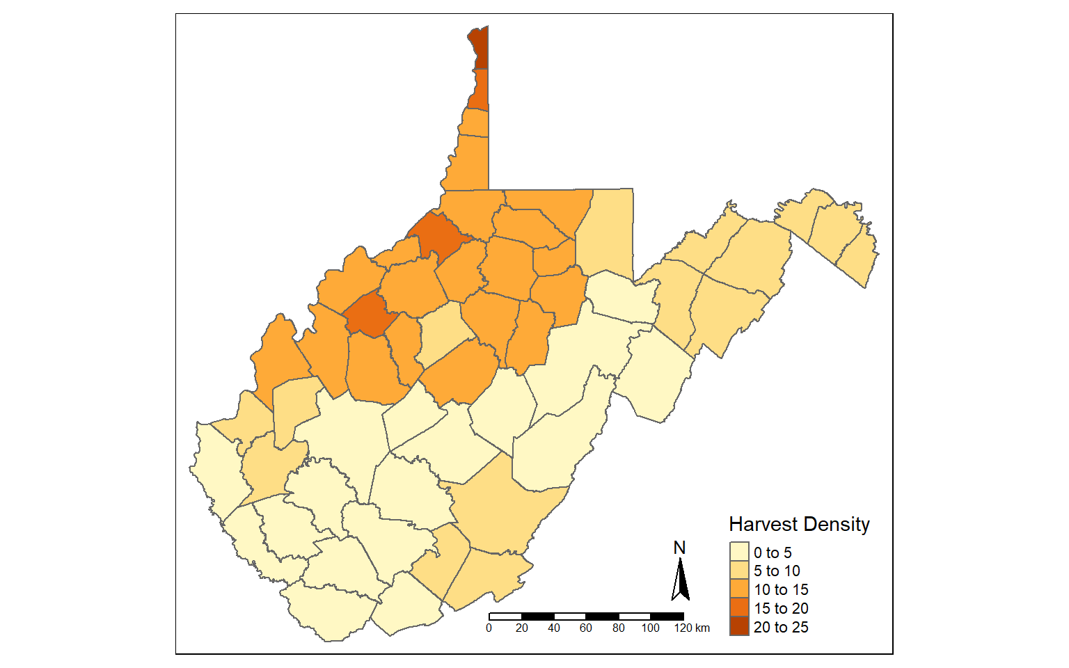

Using the filter() function, I extract out and map all counties that have a deer harvest density greater than five deer per square mile.

counties_harvest_sub <- filter(counties_harvest, DEN > 5)
tm_shape(counties_harvest_sub)+
tm_polygons(col="DEN", title = "Harvest Density")+
tm_compass()+
tm_scale_bar()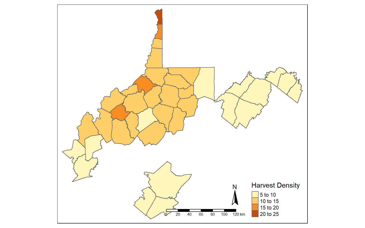

The st_area() function is used to calculate area for polygon features. The area will be returned in the map units, in this case square meters since the data are projected to a UTM coordinate system. I write the result to a new column called “hec”.

I then calculate density again using hectares as opposed to square miles.

counties_harvest$hec <- st_area(counties_harvest)*0.0001
counties_harvest <- mutate(counties_harvest, DEN2 = TOTALDEER/hec)
tm_shape(counties_harvest)+
tm_polygons(col="DEN2", title = "Harvest Density")+
tm_compass()+
tm_scale_bar()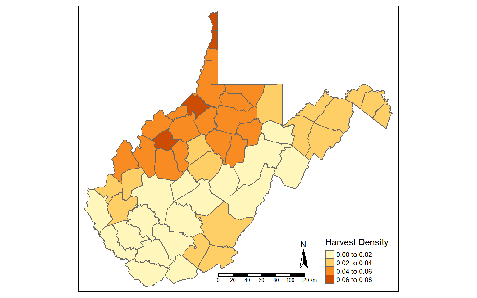

Bounding Box and Centroids

The st_bbox() function is used to extract the bounding box coordinates for a layer. It does not create a spatial feature. To convert the bounding box coordinates to a spatial feature, I use the st_make_grid() function to create a grid that covers the extent of the bounding box with a single grid cell. This is a bit of a trick, but it works well.

In the map, the bounding box for West Virginia is shown in red.

bb_wv <- st_bbox(wv_counties)

bb_wv_rec <- st_make_grid(bb_wv, n=1)

tm_shape(bb_wv_rec)+
tm_borders(col="red", lwd=2)+
tm_shape(wv_counties)+
tm_polygons(col="tan")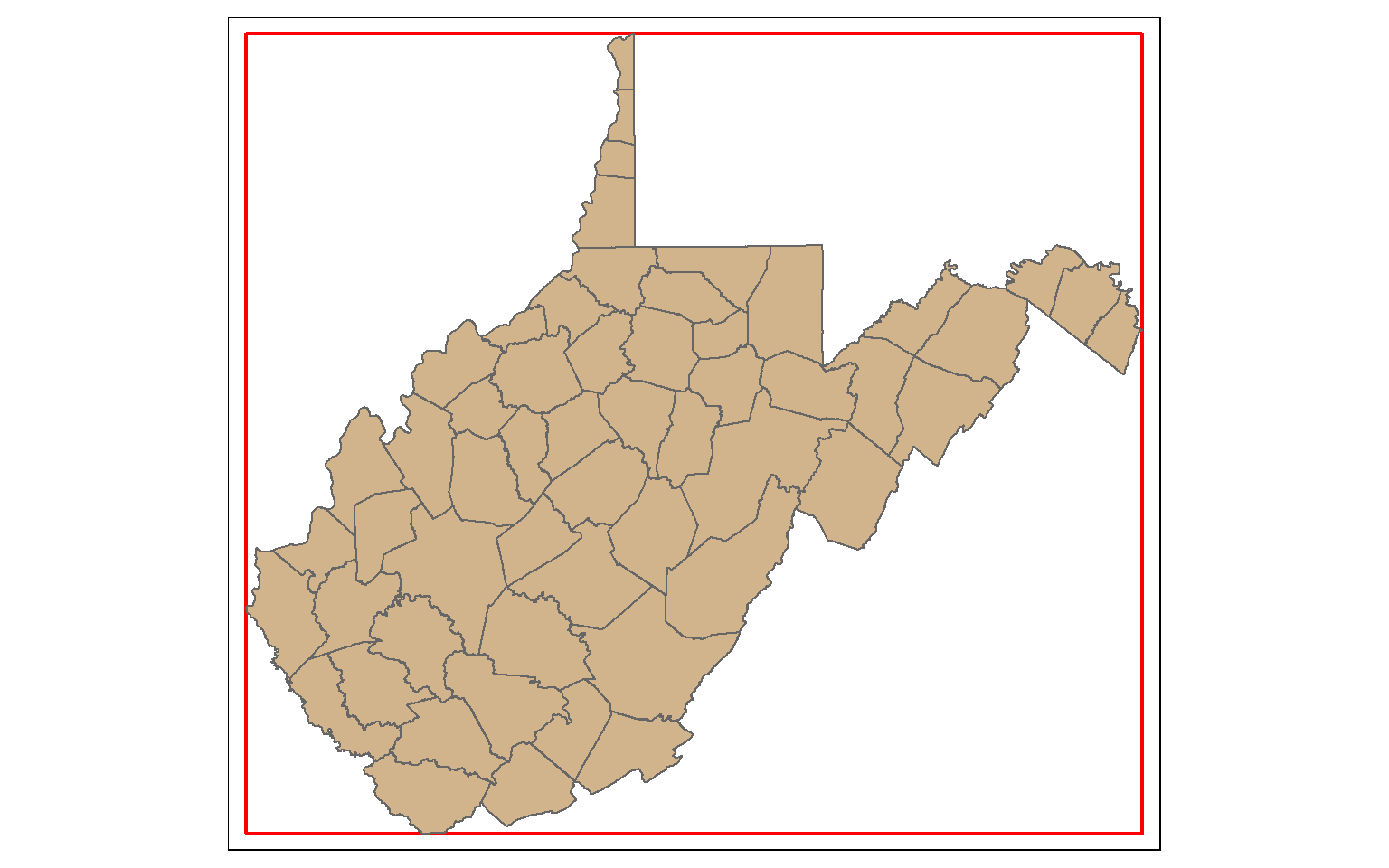

st_centroid() is used to extract the centroid coordinates of each polygon feature and returns a point geometry. Note that the centroid is not always inside of the polygon that it is the center of (for example, a “C-shaped” island or a doughnut). st_point_on_surface() provides an alternative in which a point within the polygon will be returned.

When points are generated from polygons, all the attributes are also copied, as demonstrated by calling the column names.

wv_centroids <- st_centroid(wv_counties)

tm_shape(wv_counties)+
tm_polygons(col="tan")+
tm_shape(wv_centroids)+
tm_bubbles(col="red", size=1)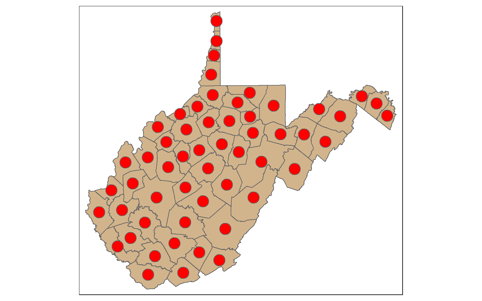

names(wv_centroids)
 [1] "AREA"       "PERIMETER"  "NAME"       "STATE"      "FIPS"      
 [6] "STATE_ABBR" "SQUARE_MIL" "POP2000"    "POP00SQMIL" "MALE2000"  
[11] "FEMALE2000" "MAL2FEM"    "UNDER18"    "AIAN"       "ASIA"      
[16] "BLACK"      "NHPI"       "WHITE"      "AIAN_MORE"  "ASIA_MORE" 
[21] "BLK_MORE"   "NHPI_MORE"  "WHT_MORE"   "HISP_LAT"   "X1900"     
[26] "X1910"      "X1920"      "X1930"      "X1940"      "X1950"     
[31] "X1960"      "X1970"      "X1980"      "X1991"      "X1992"     
[36] "X1993"      "X1994"      "X1995"      "X1996"      "X1997"     
[41] "X1998"      "X1999"      "X1990"      "X2000"      "X2001"     
[46] "X2002"      "X2003"      "X2004"      "X2005"      "X2006"     
[51] "geometry"

Voronoi or Thiessen Polygons represent the areas that are closer to one point feature than any other feature in a data set. st_voronoi() can be used to generate these polygons. However, this only works when points are aggregated to multipoint features, so I use the st_union() function to make this conversion. The result will be a GEOMETRYCOLLECTION, which can be converted back to points using st_cast(). I then extract out the polygon extents within the state using st_intersection(). We will talk about these additional methods later in this module.

So, this offers a means to convert points to polygons.

vor_poly <- st_voronoi(st_union(wv_centroids))
vor_poly2 <- st_cast(vor_poly)

wv_diss <- wv_counties %>% group_by(STATE) %>% summarize(totpop = sum(POP2000))
                                                         
vor_poly3 <- st_intersection(vor_poly2, wv_diss)

tm_shape(wv_diss)+
tm_polygons(col="tan")+
tm_shape(vor_poly3)+
tm_borders(col="red", lwd=2)+
tm_shape(wv_centroids)+
tm_bubbles(col="blue")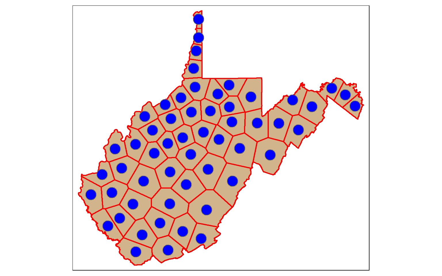

A convex hull is a bounding geometry that encompasses features without any concave angles. Think of this as stretching a rubber band around the margin points in a data set. A convex hull can be generated using the st_convex_hull() function. Similar to st_voronoi(), points must first be converted to multipoint.

ch <- st_convex_hull(st_union(wv_centroids)) 

tm_shape(wv_counties)+
tm_polygons(col="tan")+
tm_shape(wv_centroids)+
tm_bubbles(col="red", size=1)+
tm_shape(ch)+
tm_borders(col="blue", lwd=2)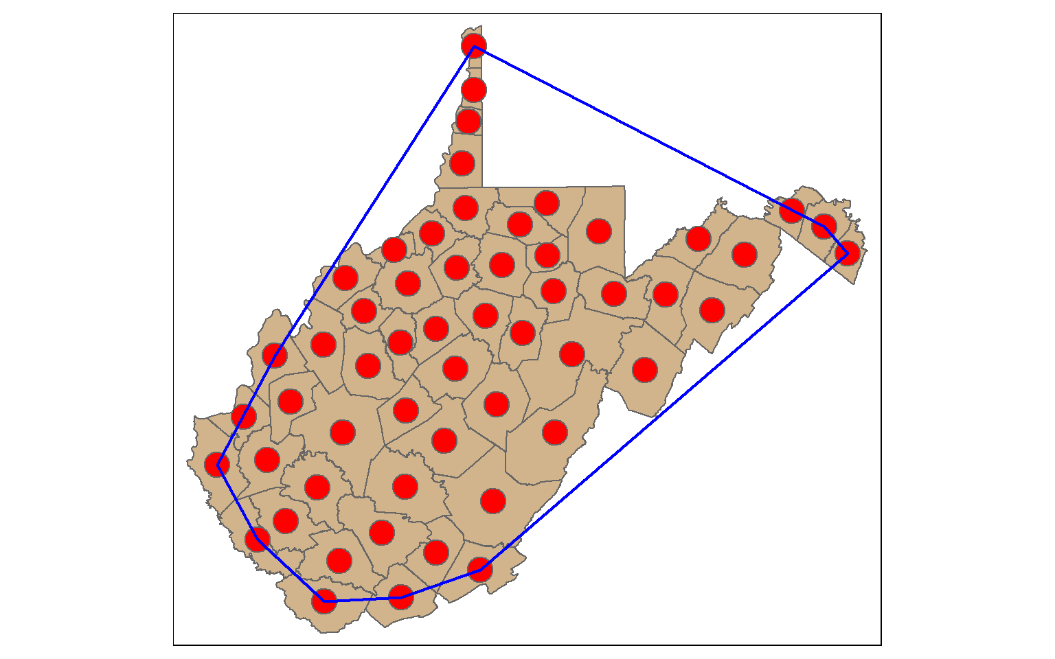

Spatial Join

In contrast to a table join, a spatial join associates features based on spatial co-occurrence as opposed to a shared or common attribute. In the next code block I am using st_join() to spatially join the cities and states. The result will be a point geometry with all the attributes from each city and the state in which it occurs.

To demonstrate this, I am symbolizing the points using the “SUB_REGION” field, which was initially attributed to the states layer.

cities2 <- st_join(us_cities, states)

tm_shape(states)+
tm_polygons(col="tan")+
tm_shape(cities2)+
tm_bubbles(col="SUB_REGION", size=.25)+
tm_layout(legend.outside = TRUE)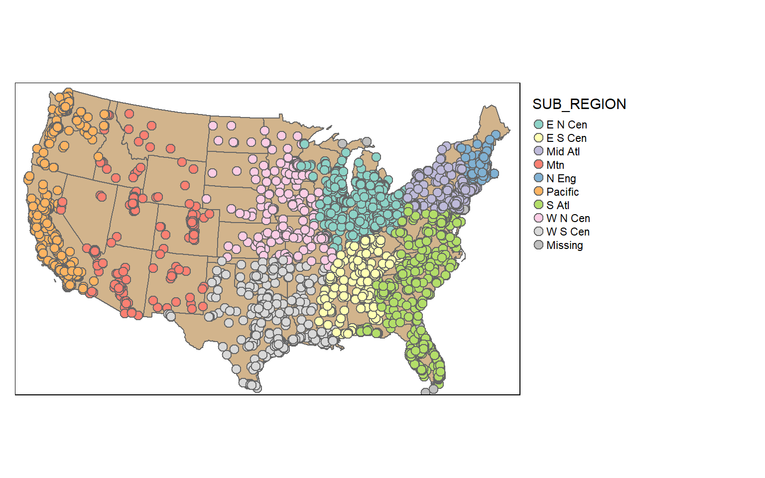

Random Sampling

Randomly sampling spatial features using dplyr is the same as randomly sampling records or rows from any data frame. In the first example, I am demonstrating simple random sampling without replacement. The replace argument is set to FALSE to indicate that I don’t want features to be selected multiple times.

The result is 100 randomly selected cities. Since this is random, you will get a different result each time you run the code.

cities_rswor <- cities2 %>% sample_n(100, replace=FALSE)

tm_shape(states)+
tm_polygons(col="tan")+
tm_shape(cities_rswor)+
tm_bubbles(col="red")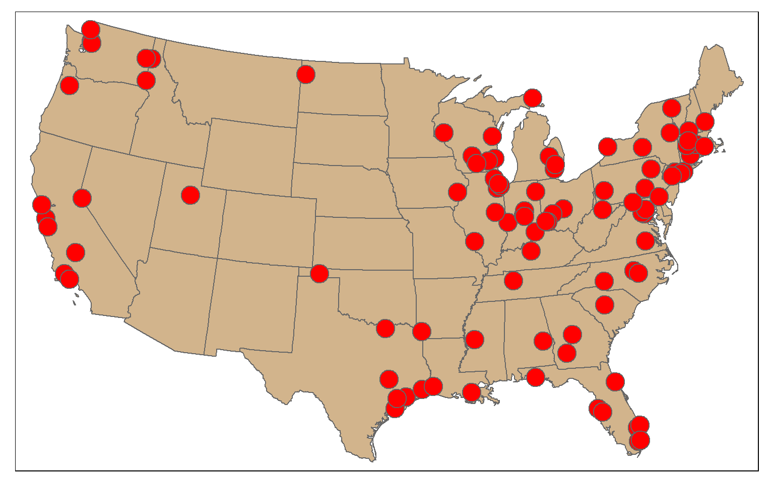

It is also possible to stratify the sampling using group_by(). Here, I am selecting 10 random cities per sub-region. To confirm this, I create a table that provides a count of selected cities by sub-region.

cities_srswor <- cities2 %>% group_by(SUB_REGION) %>% sample_n(10, replace=FALSE)

check_sample <- cities_srswor %>% group_by(SUB_REGION) %>% count()
print(check_sample)
Simple feature collection with 10 features and 2 fields
Geometry type: MULTIPOINT
Dimension:     XY
Bounding box:  xmin: -2286623 ymin: -1327888 xmax: 2034447 ymax: 1411752
Projected CRS: USA_Contiguous_Albers_Equal_Area_Conic
# A tibble: 10 x 3
   SUB_REGION     n                                                        Shape
 * <chr>      <int>                                             <MULTIPOINT [m]>
 1 E N Cen       10 ((654474.3 561320.3), (670763.6 774554.9), (740136.2 480360~
 2 E S Cen       10 ((557316.4 -266060.3), (655909.1 -774657.7), (663501.9 -768~
 3 Mid Atl       10 ((1333616 436017.9), (1344695 555703.6), (1356902 460098.9)~
 4 Mtn           10 ((-1702796 8056.471), (-1490931 -198833.6), (-1334097 45076~
 5 N Eng         10 ((1832676 906880.7), (1846182 985387.4), (1879636 639927.1)~
 6 Pacific       10 ((-2283723 441469.1), (-2148053 544673.5), (-2118827 473670~
 7 S Atl         10 ((1146800 -545145.9), (1303050 -943783.7), (1329388 -102734~
 8 W N Cen       10 ((-397138.7 417392.5), (-117141.8 61810.69), (-58878.29 676~
 9 W S Cen       10 ((-475259.2 -894949.1), (-457825.3 -523391.9), (-368632.3 -~
10 <NA>          10 ((-2286623 315506.9), (-2244551 373990.8), (-1981274 141175~
tm_shape(states)+
tm_polygons(col="tan")+
tm_shape(cities_srswor)+
tm_bubbles(col="SUB_REGION", size=.25)+
tm_layout(legend.outside = TRUE)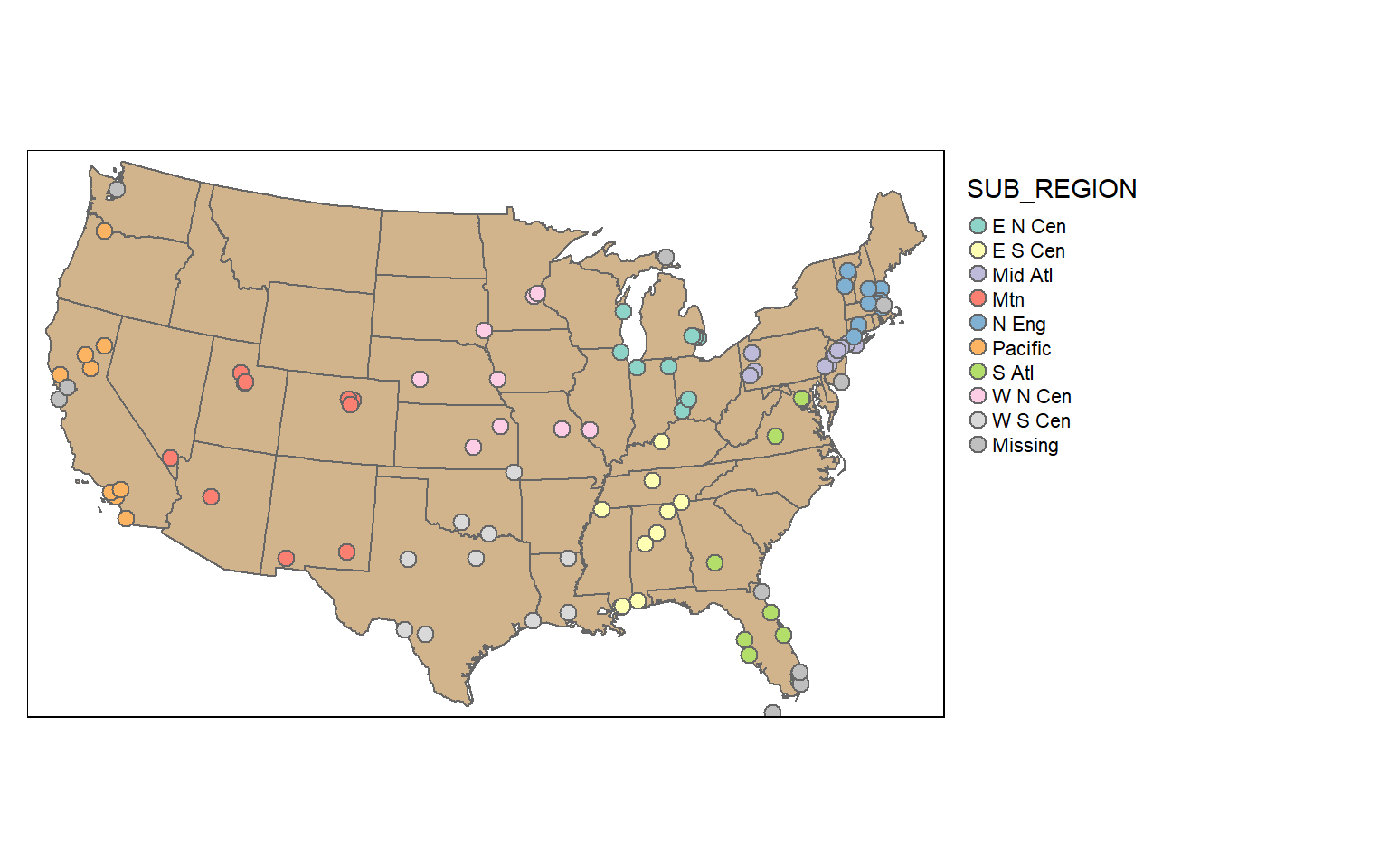

Dissolve

Dissolve is used for boundary generalization. For example, you can dissolve county boundaries to state boundaries or state boundaries to the country boundary.

In the example, I am obtaining sub-region boundaries from the state boundaries. If you would like to include a summary of some attributes relative to the dissolved features, you can include a summary() function. As an example, I am summing the population of all the states in each sub-region and writing the result to a column called “totpop”.

So, boundary generalization can be performed using only dplyr functions.

sub_regions = states %>% group_by(SUB_REGION) %>%
summarize(totpop = sum(POP2000))

tm_shape(sub_regions)+
tm_polygons(col="SUB_REGION")+
tm_layout(legend.outside = TRUE)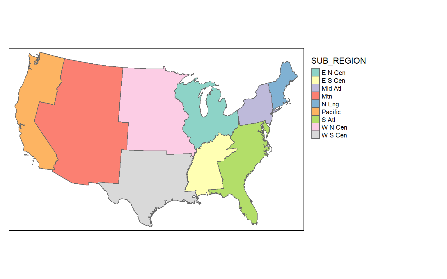

This is another example of dissolve where I have generated the West Virginia state boundary from the county boundaries. Since all counties have the same value in the “STATE” field, a single feature is returned. I have also summed the population for each county, which will result in the total state population.

wv_diss <- wv_counties %>% group_by(STATE) %>%
summarize(totpop = sum(POP2000))

tm_shape(wv_diss)+
tm_polygons(col="tan")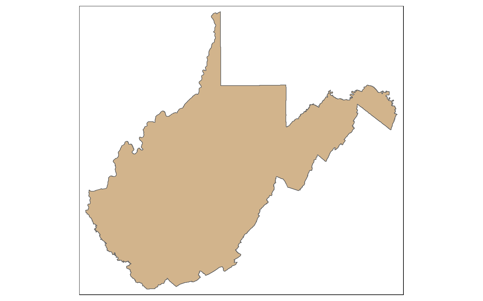

Buffer

Proximity analysis relates to finding features that are near to other features. A buffer represents the area that is within a defined distance of an input feature. Buffers can be generated for points, lines, and polygons. The result will always be a polygon or area.

In the example, I have created polygon buffers that encompass all areas within 20 km of the mapped interstates using the st_buffer() function. The buffer distance is defined in the map units, in this case meters.

us_inter_20km <- st_buffer(us_inter, 20000)

tm_shape(states) +
tm_polygons(col="tan")+
tm_shape(us_inter_20km)+
tm_polygons(col="red", alpha=.6)+
tm_shape(us_inter)+
tm_lines(lwd=1, col="black")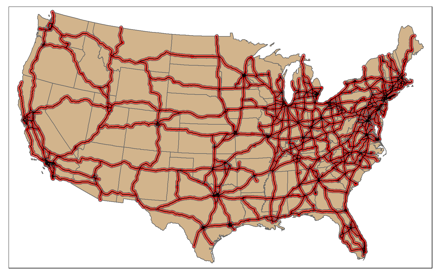

Clip and Intersect

Clip and intersect are used to extract features within another feature or return the overlapping extent of multiple features. Think of this as a spatial AND.

In this example I am intersecting the circle and triangle. The result will be the area that occurs in both the circle and the triangle (shown in red).

All attributes from both features will be returned, as demonstrated by calling glimpse() on the output. The table contains both the “C” and “T” fields, which came from the circle and triangle, respectively.

So, st_intersection() is equivalent to the Intersect Tool in ArcGIS. However, it can also be used to perform a clip, as the geometric result is the same.

isect_example <- st_intersection(circle, triangle)

tm_shape(ext)+
tm_borders(col="black")+
tm_shape(circle)+
tm_polygons(col="#0D5C86")+
tm_shape(triangle)+
tm_polygons(col="#67B38C")+
tm_shape(isect_example)+
tm_polygons(col="#FD694F")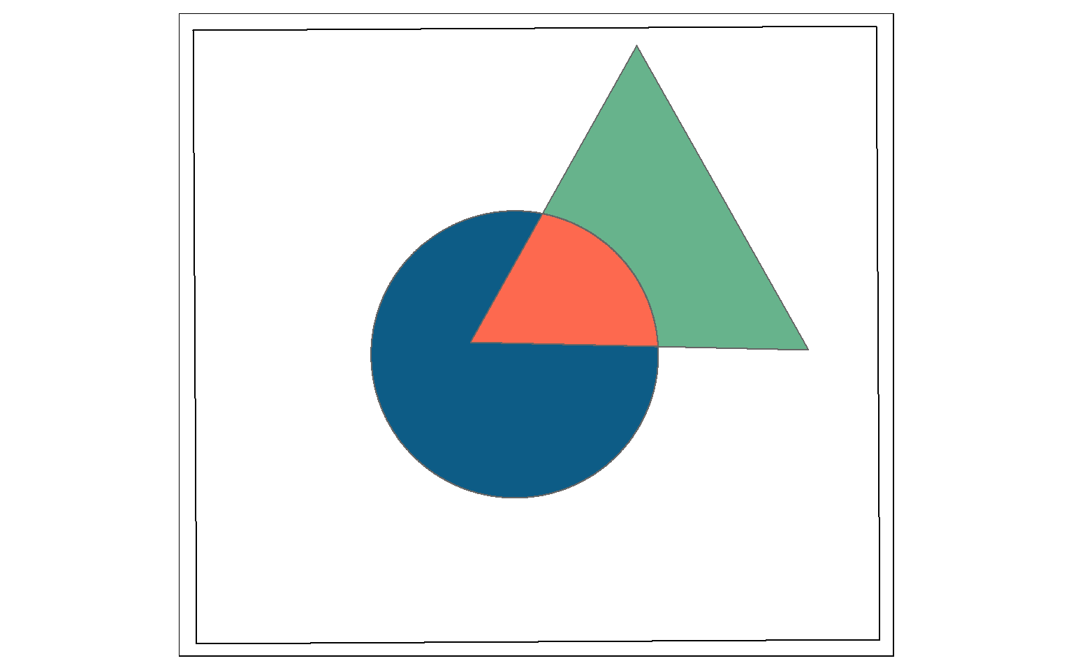

glimpse(isect_example)
Rows: 1
Columns: 6
$ Id       <int> 0
$ C        <chr> "C"
$ Id.1     <int> 0
$ T        <chr> "T"
$ area     <dbl> 7360.591
$ geometry <POLYGON [m]> POLYGON ((587509.3 4395549,...

In this example, I am using st_intersection(), the interstate buffers, and the tornado points to find all tornadoes that occurred within 20 km of an interstate. So, buffer and intersection can be combined to find features within a specified distance of other features.

isect_example <- st_intersection(torn, us_inter_20km)

tm_shape(states) +
tm_polygons(col="tan")+
tm_shape(us_inter_20km)+
tm_polygons(col="red", alpha=.6)+
tm_shape(us_inter)+
tm_lines(lwd=1, col="black")+
tm_bubbles(col="black")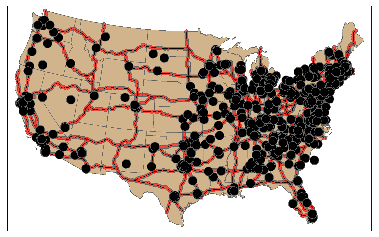

Union, Erase, and Symmetrical Difference

st_union() from sf is a bit different from the Union Tool in ArcGIS. Instead of returning the unioned area with all boundaries, the features are merged to a single feature with no internal boundaries. In the example, the full spatial extent of the circle and triangle is returned as a single feature. Similar to st_inersection(), all attributes are maintained. Think of this as a spatial OR.

union_example <- st_union(circle, triangle, by_feature=TRUE)

tm_shape(ext)+
tm_borders(col="black")+
tm_shape(union_example)+
tm_polygons(col="#FD694F")

st_difference() will return the portion of the the first geometric feature that is not in the second. This is similar to the Erase Tool in ArcGIS. This is a spatial NOT: Circle NOT Triangle. The result is the portion of the circle shown by the dotted red extent displayed in the map below.

erase_example <- st_difference(circle, triangle)
tm_shape(ext)+
tm_borders(col="black")+
tm_shape(circle)+
tm_polygons(col="#0D5C86")+
tm_shape(triangle)+
tm_polygons(col="#67B38C")+
tm_shape(erase_example)+
tm_polygons(col="#FD694F", border.col="red", lty=5, lwd=4, alpha=.6)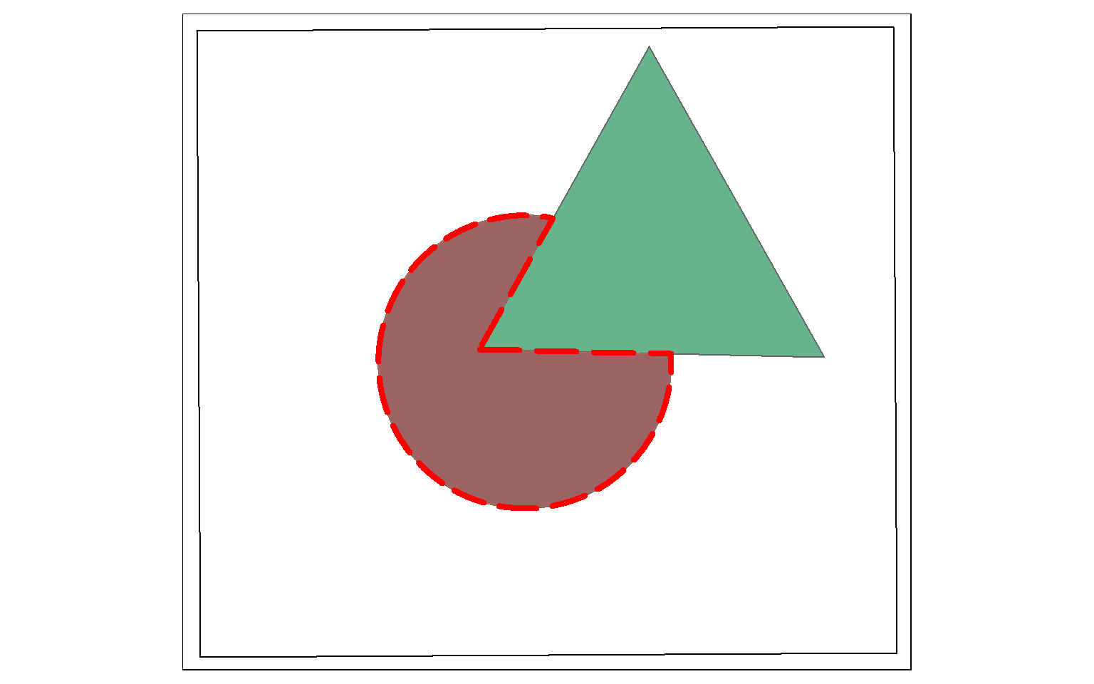

Symmetrical difference is a spatial XOR: Circle OR Triangle, excluding Circle AND Triangle. So, the result will be the area in either the circle or the triangle, but not the area in both as demonstrated in the example below.

sym_diff_examp <- st_sym_difference(circle, triangle)

tm_shape(ext)+
tm_borders(col="black")+
tm_shape(sym_diff_examp)+
tm_polygons(col="#FD694F")

Points in Polygons

You can count the number of point features occurring in polygons using sf and dplyr. In the example, I am counting the number of cities in each state using the method outlined below.

First, I use st_join() to join the cities and states using a spatial join. This will result in a point geometry where each point has the city and state attributes.
I then use group_by() and count() from dplyr to count the number of cities by state.
I use st_drop_geometry() to remove the geometric information from the output and return just the aspatial data.
I join the table back to the state boundaries using the common “STATE_NAME” field and a table join.

Once this process is complete, I then map the resulting counts. This entire process is completed using only sf and dplyr.

cities_in_state <- st_join(us_cities, states)
cities_cnt <- cities_in_state %>% group_by(STATE_NAME) %>% count()

cities_cnt <- st_drop_geometry(cities_cnt)

state_cnt <- left_join(states, cities_cnt, by="STATE_NAME")

tm_shape(state_cnt) +
tm_polygons(col="n", title = "Number of Cities")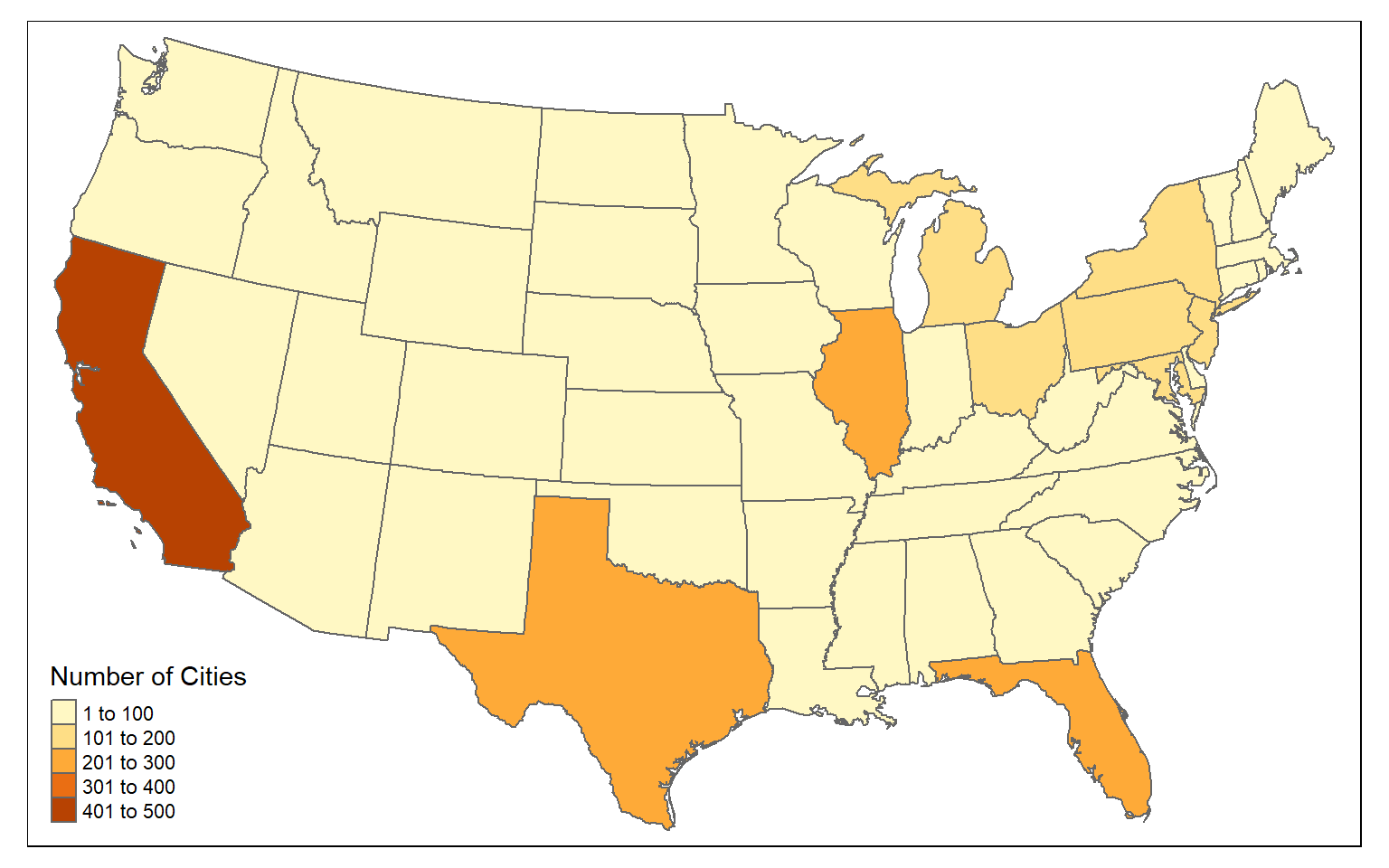

Length of Lines in Polygons

You can also sum the length of lines by polygon. In the example, I am summing the length of interstates by state.

First, I intersect the interstates and states using st_intersection() to obtain a line geometry where the interstates have been split along state boundaries and now have the state attributes.
I then use st_length() to calculate the length of each line segment. I cannot use the original length field because this will not reflect the length after the interstates are split along state borders. I divide by 1,000 to obtain the measure in kilometers as opposed to meters.
I then group the lines by state and sum the length using dplyr.
I remove the geometry from the result.
I join the result back to the state boundaries using left_join() and the common “STATE_NAME” field.

I then map the results using tmap. Again, this was accomplished using only sf and dplyr.

us_inter_isect <- st_intersection(us_inter, states)
us_inter_isect$ln_km <- st_length(us_inter_isect)/1000
state_ln <- us_inter_isect %>% group_by(STATE_NAME) %>% summarize(inter_ln = sum(ln_km))

state_ln <- st_drop_geometry(state_ln)

state_inter_ln <- left_join(states, state_ln, by="STATE_NAME")

tm_shape(state_inter_ln)+
tm_polygons(col="inter_ln", title= "Length (km)")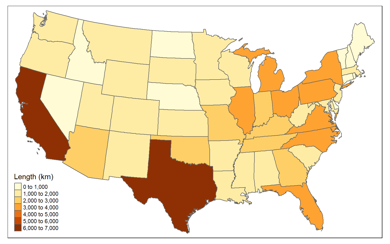

For a fairer comparison, it would make sense to calculate the density of interstates as length of interstates in kilometers per square kilometer. Again, this can be accomplished using only sf and dplyr.

state_inter_ln$sq_km <- st_area(state_inter_ln)*1e-6

state_inter_ln <- state_inter_ln %>% mutate(int_den = inter_ln/sq_km)

tm_shape(state_inter_ln)+
tm_polygons(col="int_den", style="quantile", title="km per square km")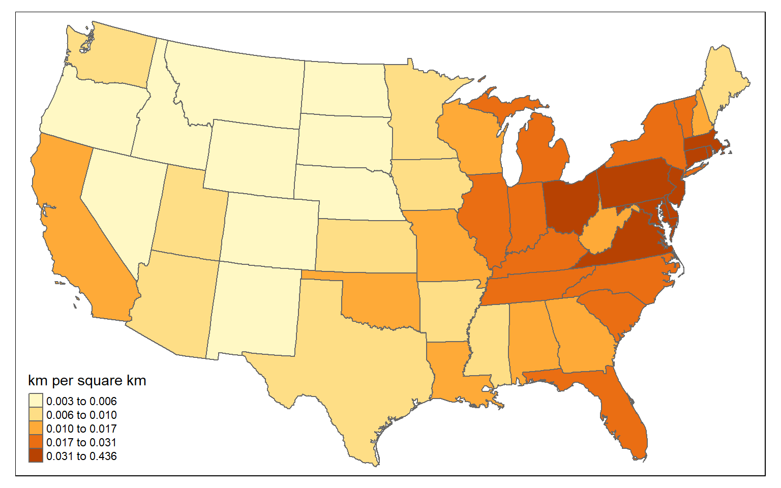

Simplify Polygons

The st_simplify() function can be used to simplify or generalize features. Higher values for dTolerance will result in more simplification. Topology can be preserved using the perserveTopology argument.

state_100000 <- st_simplify(states, dTolerance=100000, preserveTopology = TRUE)
tm_shape(state_100000)+
tm_polygons(col="tan")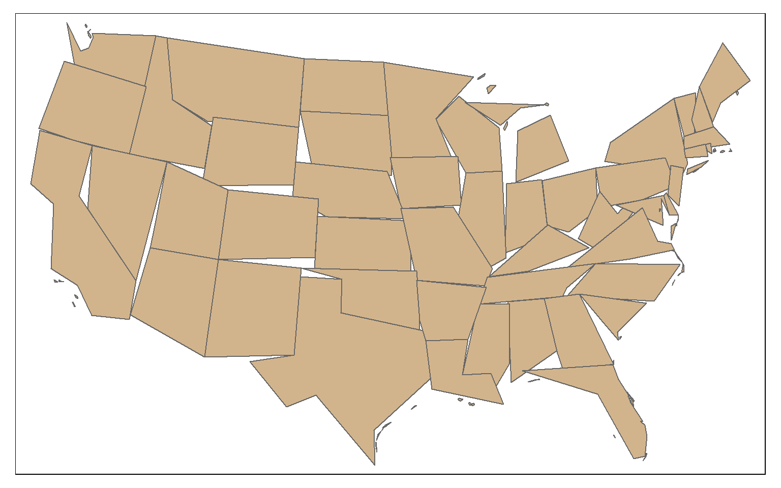

In this second example, topology is not preserved.

state_100000 <- st_simplify(states, dTolerance=100000, preserveTopology = FALSE)
tm_shape(state_100000)+
tm_polygons(col="tan")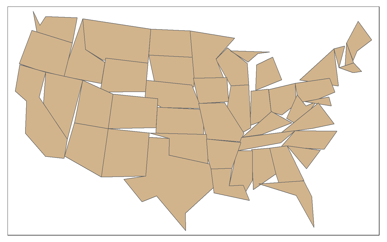

This is a simplification of the West Virginia boundary using a tolerance of 10,000 meters with topology preserved.

wv_bound <- states %>% filter(STATE_NAME=="West Virginia")
wv_simp <- st_simplify(wv_bound, dTolerance=10000, preserveTopology = TRUE)
tm_shape(wv_simp)+
tm_polygons(col="tan")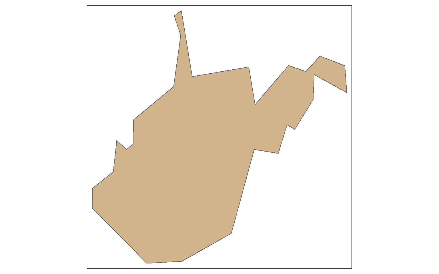

Random Points in Polygons

Random points can be generated within polygons using the st_samples() function. In the example, I am generating 400 random points across the country. Since this is random, you will get a different result if you re-execute the code. You can also set the type argument to “regular” to obtain a regular as opposed to random pattern.

pnt_sample <- st_sample(states, 400, type="random")
tm_shape(states)+
tm_polygons(col="tan")+
tm_shape(pnt_sample)+
tm_bubbles(col="black")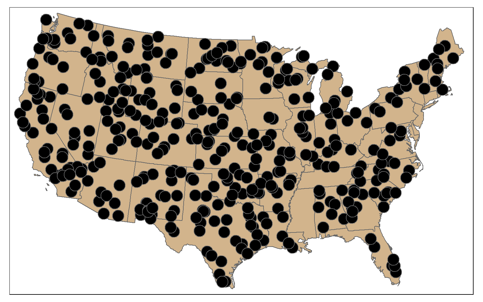

By combining st_sample() with group_by() you can stratify the sample based on a category. In the example, I am extracting 10 random points in each state.

pnt_sample2 <- states %>% group_by(STATE_NAME) %>% st_sample(rep(10, 49), type="random")
tm_shape(states)+
tm_polygons(col="tan")+
tm_shape(pnt_sample2)+
tm_bubbles(col="black")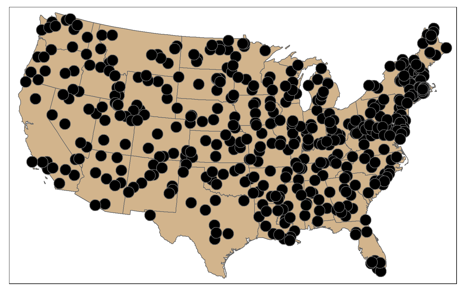

Tessellation

st_make_grid() can be used to produce a rectangular grid tessellation over an extent. Here, I am extracting the bounding box for the states data. I then create a rectangle from the bounding box using st_make_grid(), as already demonstrated above. I then create a new grid of 10 by 10 cells within this extent also using st_make_grid().

states_bb <- st_bbox(states)
states_bb_rec <- st_make_grid(states_bb, n=1)
us_grid <- st_make_grid(states_bb_rec, n=c(10, 10))
tm_shape(states)+
tm_polygons(col="tan")+
tm_shape(us_grid)+
tm_polygons(col="red", alpha=.2, border.col="black", lwd=2)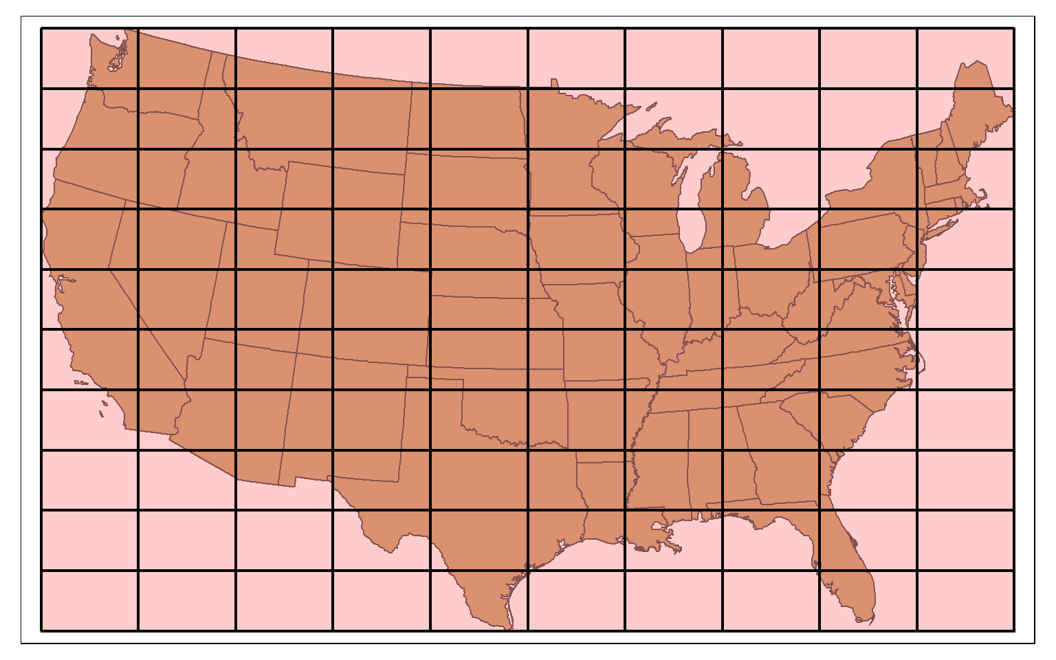

A hexagonal tessellation can be obtained by setting the square argument in st_make_grid() to FALSE.

states_bb <- st_bbox(states)
states_bb_rec <- st_make_grid(states_bb, n=1)
us_hex <- st_make_grid(states_bb_rec, n=c(10, 10), square=FALSE)
tm_shape(states)+
tm_polygons(col="tan")+
tm_shape(us_hex)+
tm_polygons(col="red", alpha=.2, border.col="black", lwd=2)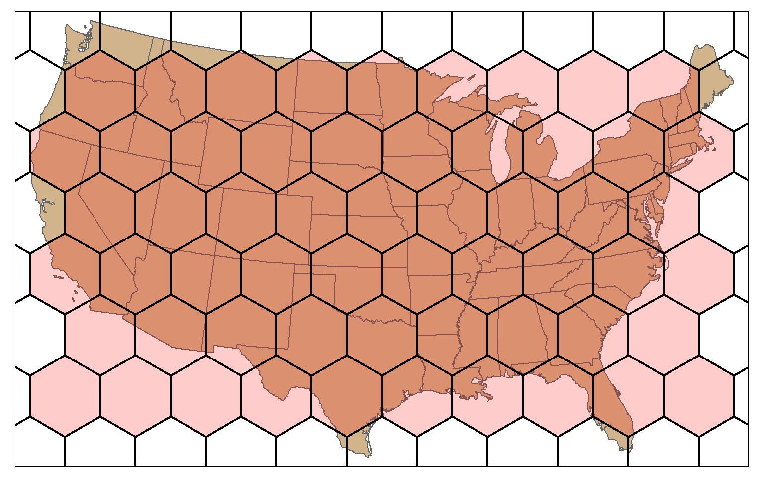

The tessellation result can then be clipped to the extent of the polygon data using st_intersection(). In this example, I am using the country boundary, created by dissolving the state boundaries, to clip the tessellation.

us_diss <- st_union(states)
us_hex2 <- st_intersection(us_hex, us_diss)
tm_shape(states)+
tm_polygons(col="tan")+
tm_shape(us_hex2)+
tm_polygons(col="red", alpha=.2, border.col="black", lwd=2)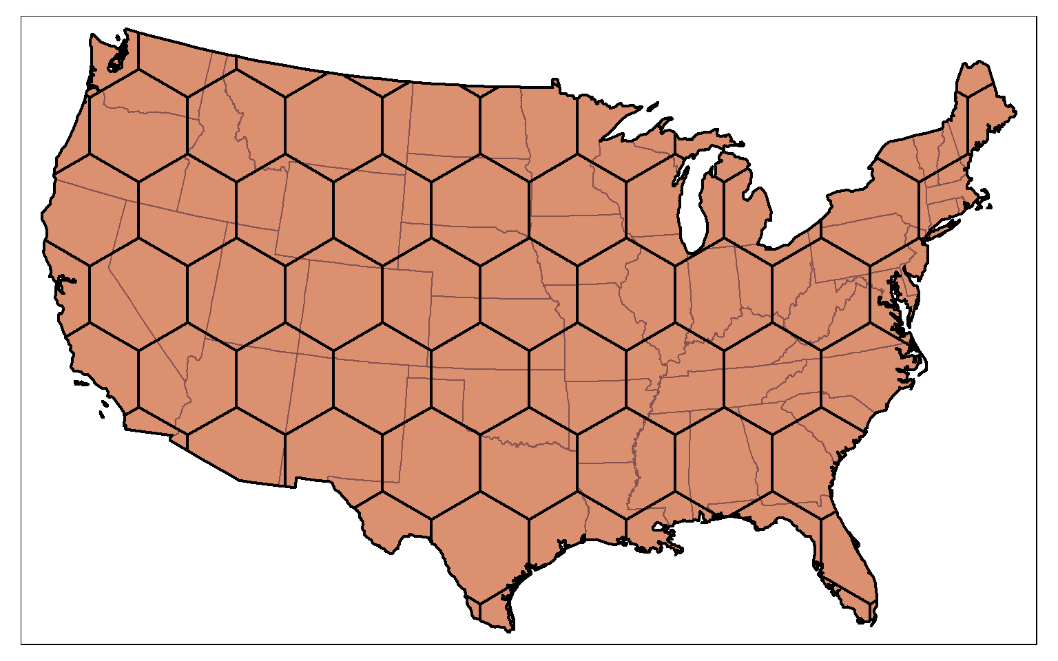

Concluding Remarks

Again, I’ve tried to focus on common geoprocessing and vector analysis techniques here. You will likely run into specific issues that will require different techniques. However, I think you will find that the examples provided can offer a starting point for other analyses.

I also focused on dplyr and sf. However, there are other packages available for working with vector data. Many rely on sp, so you need to know how to convert between sp and sf types. You can save the results of your analyses to permanent files using the methods discussed in the spatial data module.

Now that you have studied vector-based spatial analysis, you are ready to investigate working with and analyzing raster data in R.