Interpretable Machine Learning with Explainable Boosting Machine
Although machine learning algorithms, such as support vector machines and random forest, often outperform simpler methods, such as linear regression or logistic regression, they are less interpretable. For example, a random forest model consists of a large set of decision trees, and it is not easy to visualize the model. In contrast, a linear regression model is summarized by a single equation (e.g., y = mx + b). Machine learning methods are often described as "black box" methods.
In some situations it is important to have a clear interpretation of the output obtained, such as in law, medicine, and finance. Methods have been developed to add interoperability to black box methods including variable importance estimates, partial dependency plots, local interpretable model-agnostic explanations (LIME), and shapely additive explanations (SHAP). However, as opposed to implementing methods to make a black box model more interpretable, it might be preferable to use a method that is inherently interpretable.
Methods that are generally interpretable include linear regression, multiple linear regression, generalized linear models (e.g., logistic regression), and generalized additive models (GAMs). Recently, GAMs have been augmented to offer both interpretability and strong predictive performance with the introduction of the explainable boosting machine (EBM) method. This method is based on the generalized additive models plus interactions (GA2M) algorithm, which was introduced by Lou et al. (2013). EBM, which was developed by Microsoft Research, provides a fast implementation of this method. Within Python, it is implemented in the interpretml library. Here is a link to the GitHub page.
EBM builds upon or augments generalized additive models (GAMs), which take the general form:
ŷ = β0 + f1(x1) + f2(x2) + f3(x3) + …… + fi(xi)
The predicted value (ŷ) is estimated using a y-intercept (β0) and a series of additive terms consisting of learned functions (fi) and associated predictor variable values. Essentially, the coefficients (βi) in a multiple linear regression model are replaced with learned functions (fi) that are not confined to a linear relationship. The model is additive because separate functions are learned for each predictor variable independently, which allows for an examination of the effect of each predictor variable separately. In order to apply GAMs to binary classification problems, class logits are predicted as opposed to a continuous variable:
log((p(x))/(1-p(x))) = β0 + f1(x1) + f2(x2) + f3(x3) + ……. + fi(xi)
In this equation, p represents the probability of the sample belonging to the positive class, which is assigned a value of 1 while the negative class is assigned a value of 0.
Expanding upon traditional GAMs, the EBM method relies on the approximation of functions associated with each predictor variable using many shallow decision trees created with gradient boosting to iteratively improve model performance. More specifically, shallow decision tree generation, learning, and gradient updates are performed using a single predictor variable at a time in a round-robin fashion with a low learning rate. Due to the low learning rate, only small updates to the model are made with the addition of each tree. This requires the model to be built by iterating through the training data over thousands of boosting iterations in which each tree only uses one predictor variable. The algorithm developers argue that the low learning rate reduces the influence of the order in which features are used while iteratively cycling through the predictor variables using a round-robin method minimizes the impact of co-linearity to maintain interpretability. To take into account interactions between predictor variables, two-dimensional functions (fij(xi, xj)) can be learned to relate the response variable to pairs of predictor variables. The subset of available interactions included are selected using the FAST method proposed by Lou et al. (2013) that ranks all pairs of predictor variables.
Once an ensemble of decision trees is trained using gradient boosting, all trees produced for a single predictor variable are used to predict the training samples and build the function associated with each feature. Once the trees are used to build the function for each predictor variable, they are no longer needed, simplifying inference to new data. Thus, the function associated with each predictor variable or interaction is derived from the large set of shallow trees. For binary classification and associated class probabilities, the final prediction is derived by adding all scores (i.e., the effect of each included factor on the predicted logits for the positive class) estimated using each predictor variable and included interactions with the use of a link function to adapt to specific tasks (i.e., regression vs. classification).
For the global model, results include (1) graphic output of the functions for each predictor variable and each included two-dimensional interaction and (2) an assessment of variable importance for each predictor variable and interaction term. For binary classification problems specifically, the predicted relationship between the predictor variable and the dependent variable is obtained by graphing the values of the predictor variable to the x-axis and the associated prediction or score to the y-axis. For included two-dimensional interactions, each variable will be mapped to an axis and the resulting prediction or score will be presented as a heat map within the two-dimensional space. As a result, all components of the model can be represented graphically, which the algorithm originators cite as the key characteristic of an interpretable model. Larger scores indicate that the model associates those ranges of predictor variable values with a higher likelihood of occurrence of the positive class whereas lower values are associated with a lower likelihood or probability of occurrence. In the current InterpretML implementation of EBM, variable importance is estimated as the average absolute value of the predicted score provided by the predictor variable when predicting each feature in the training set. Features that have larger magnitudes of feature function scores will generally show greater importance.
Once a new sample is predicted, such as a new pixel or aggregating unit, the score associated with each predictor variable can be obtained to aid in interpreting what characteristics resulted in the prediction. Features that have larger magnitude positive or negative scores have a larger influence in the resulting prediction than features that had scores nearer to zero.
More information about the EBM algorithm can be found in the associated documentation, linked above, and the following publications.
Lou, Y., Caruana, R., Gehrke, J. and Hooker, G., 2013, August. Accurate intelligible models with pairwise interactions. In Proceedings of the 19th ACM SIGKDD international conference on Knowledge discovery and data mining (pp. 623-631).
Nori, H., Jenkins, S., Koch, P. and Caruana, R., 2019. Interpretml: A unified framework for machine learning interpretability. arXiv preprint arXiv:1909.09223.
Caruana, R., Lou, Y., Gehrke, J., Koch, P., Sturm, M. and Elhadad, N., 2015, August. Intelligible models for healthcare: Predicting pneumonia risk and hospital 30-day readmission. In Proceedings of the 21th ACM SIGKDD international conference on knowledge discovery and data mining (pp. 1721-1730).
As an example application in the geospatial sciences, have a look at the following paper that investigates the probabilistic prediction of slope failure occurrence. Most of the text presented above was modified from this publication.
Maxwell, A.E., M. Sharma, and K.A. Donaldson, 2021. Explainable boosting machines for slope failure spatial predictive modeling, Remote Sensing, 13(24): 1-27. https://doi.org/10.3390/rs13244991.
In this module, I will demonstrate the interpretml Python library and the included EBM model for predicting a binary outcome. Specifically, we will investigate the famous Titanic dataset to predict whether a passenger survived or did not survive based on a set of predictor variables:
- Pclass: whether the passenger was traveling in first, second, or third class
- Sex: male or female
- Age: age of passenger
- Siblings/Spouses Aboard: number of siblings aboard the ship
- Parents/Children Aboard: number of parents or children aboard the ship
- Fare: price paid for fare
After working through this module you will be able to:
- prepare data for input into the EBM algorithm
- train the EBM algorithm
- interpret the obtained global EBM model and local predictions
Preparing and Exploring Data
First, I load in the required libraries or modules including numpy, pandas, matplotlib, and seaborn. I also read in specific components from the interpretml and sklearn (or, scikit-learn) libraries.
Instructions for installing interpretml into an Python environment are provided within the package documentation.
I next read in the dataset, which is a CSV file, using read_csv() from pandas.
import numpy as np
import pandas as pd
from interpret.glassbox import ExplainableBoostingClassifier
from interpret import show
from sklearn.model_selection import train_test_split
from sklearn.metrics import confusion_matrix, classification_report, ConfusionMatrixDisplay

import matplotlib.pyplot as plt
%matplotlib inline
import seaborn as sns
titanic = pd.read_csv("D:/mydata/titanic.csv")
print(titanic.head())
   Survived  Pclass                                               Name  \
0         0       3                             Mr. Owen Harris Braund
1         1       1  Mrs. John Bradley (Florence Briggs Thayer) Cum...
2         1       3                              Miss. Laina Heikkinen
3         1       1        Mrs. Jacques Heath (Lily May Peel) Futrelle
4         0       3                            Mr. William Henry Allen

      Sex   Age  Siblings/Spouses Aboard  Parents/Children Aboard     Fare
0    male  22.0                        1                        0   7.2500
1  female  38.0                        1                        0  71.2833
2  female  26.0                        0                        0   7.9250
3  female  35.0                        1                        0  53.1000
4    male  35.0                        0                        0   8.0500
Before we proceed, printing the data types of the provided columns suggests some issues. The "Survived" column has been read in as an integer (0 = Not Survived, 1 = Survived). However, we would like it to be treated as a nominal variable. Similarly, the "Pclass" column should also be treated as a nominal variable.
To address these issues, pandas is used to change the data types of these columns. I also rename the "Siblings/Spouses Aboard" and "Parents/Children Aboard" columns so that the names are shorter and simpler.
Next, I check to make sure there are no missing values using is.null(). This suggests that there are no missing values.
To assess how balanced the dataset is, I then print the number of samples by group. There are 545 records for passengers that did not survive (code 0) and 342 for those that did survive (code 1). So, the dataset is not balanced, but there is a reasonable number of samples per class. So, we won't worry about issues of data imbalance.
print(titanic.dtypes)
Survived                     int64
Pclass                       int64
Name                        object
Sex                         object
Age                        float64
Siblings/Spouses Aboard      int64
Parents/Children Aboard      int64
Fare                       float64
dtype: object
titanic.Survived = titanic.Survived.astype(str)
titanic.Pclass = titanic.Pclass.astype(str)
titanic.rename({"Siblings/Spouses Aboard": "Siblings", "Parents/Children Aboard": "Parents"}, axis=1, inplace=True)
print(titanic.dtypes)
Survived     object
Pclass       object
Name         object
Sex          object
Age         float64
Siblings      int64
Parents       int64
Fare        float64
dtype: object
titanic.isnull().values.any()
False
titanic.groupby(['Survived']).size()
Survived
0    545
1    342
dtype: int64
Next, I split the y variable and predictor variables into separate DataFrames. I exclude the field that is not being used in the model (i.e., "Name"). I then use the train_test_split() function from sklearn. I reserve 33% of the data for testing and I stratify on the "Survived" data column (did or did not survive) in order to maintain an adequate number of samples from each class in the data partitions. I then print the number of samples per class in each data division.
survival = titanic['Survived'].to_frame()
preds = titanic[['Pclass', 'Sex', 'Age', 'Siblings', 'Parents', 'Fare']]
X_train, X_test, y_train, y_test = train_test_split(preds,
survival, test_size=0.33, random_state=42, stratify=survival)
print(y_train.groupby(['Survived']).size())
print(y_test.groupby(['Survived']).size())
Survived
0    365
1    229
dtype: int64
Survived
0    180
1    113
dtype: int64
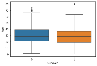
Before training a model, I explore the data using graphs and contingency tables.
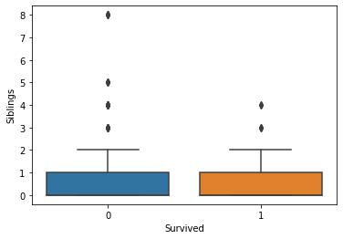
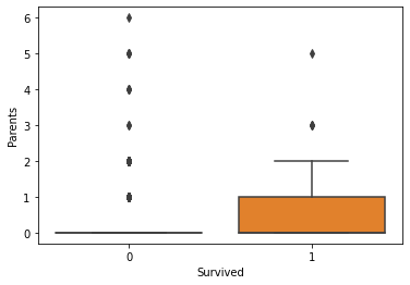
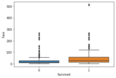
Generally, the age and number of siblings were not very different between the survivor vs. victim groups. However, survivors tended to have a larger number of parents and/or children onboard. Paying more for the voyage tended to correlate with a higher likelihood of survival. First-class passengers and women were more likely to survive than lower-class passengers and men.
fig, axs = plt.subplots(1, 1)
sns.boxplot(ax=axs, x="Survived", y="Age", data=titanic)
plt.show(fig)
fig, axs = plt.subplots(1, 1)
sns.boxplot(ax=axs, x="Survived", y="Siblings", data=titanic)
plt.show(fig)
fig, axs = plt.subplots(1, 1)
sns.boxplot(ax=axs, x="Survived", y="Parents", data=titanic)
plt.show(fig)
fig, axs = plt.subplots(1, 1)
sns.boxplot(ax=axs, x="Survived", y="Fare", data=titanic)
plt.show(fig)
pd.crosstab(titanic.Survived, titanic.Pclass)
| Pclass | 1 | 2 | 3 |
|---|---|---|---|
| Survived | |||
| 0 | 80 | 97 | 368 |
| 1 | 136 | 87 | 119 |
pd.crosstab(titanic.Survived, titanic.Sex)
| Sex | female | male |
|---|---|---|
| Survived | ||
| 0 | 81 | 464 |
| 1 | 233 | 109 |
Train and Explore Model
I am now ready to train the model. The syntax for training the model using the ExplainableBoostingClassifier() function is very similar to training a model using sklearn. Here, I am using the default hyperparameter settings.
ebm = ExplainableBoostingClassifier()
ebm.fit(X_train, y_train)
ExplainableBoostingClassifier(feature_names=['Pclass', 'Sex', 'Age', 'Siblings',
                                             'Parents', 'Fare', 'Pclass x Sex',
                                             'Age x Siblings', 'Sex x Age',
                                             'Siblings x Fare', 'Pclass x Age',
                                             'Age x Parents', 'Age x Fare',
                                             'Sex x Fare', 'Pclass x Fare',
                                             'Sex x Siblings'],
                              feature_types=['categorical', 'categorical',
                                             'continuous', 'continuous',
                                             'continuous', 'continuous',
                                             'interaction', 'interaction',
                                             'interaction', 'interaction',
                                             'interaction', 'interaction',
                                             'interaction', 'interaction',
                                             'interaction', 'interaction'])
Once the model is fit, the global model can be interpreted by exploring (1) variable importance, (2) functions associated with each predictor variable, and (3) heat maps associated with included interactions. Here, I will discuss some key findings.
First, the sex and passenger class were the most important variables in the model. Generally, females and/or passengers traveling in first-class were more likely to survive, which reinforces our graphical exploration above. The included interaction terms were generally of low importance. Please take some time to explore the variable importance plot and individual plots for each variable or interaction term. Note the difference between the functions associated with nominal and continuous predictor variables and that the interaction terms are visualized using a heat map. Effectively, these graphs represent all components of the model visually.
The next set of graphs provide the associated scores for each predictor variable and included interactions for each individual data point. This allows the user to explore what characteristics for a specific passenger resulted in the obtained prediction. Larger, positive values for a variable indicate that that predictor variable was predictive of survival. In contrast, negative values indicate that the predictor variable suggested not survival for that passenger. Each plot includes the predicted and actual classes along with the associated probability.
ebm_global = ebm.explain_global()
show(ebm_global)
C:\Users\amaxwel6\Anaconda3\envs\wvview\lib\site-packages\interpret\visual\udash.py:5: UserWarning:
The dash_html_components package is deprecated. Please replace
`import dash_html_components as html` with `from dash import html`
  import dash_html_components as html
C:\Users\amaxwel6\Anaconda3\envs\wvview\lib\site-packages\interpret\visual\udash.py:6: UserWarning:
The dash_core_components package is deprecated. Please replace
`import dash_core_components as dcc` with `from dash import dcc`
  import dash_core_components as dcc
C:\Users\amaxwel6\Anaconda3\envs\wvview\lib\site-packages\interpret\visual\udash.py:7: UserWarning:
The dash_table package is deprecated. Please replace
`import dash_table` with `from dash import dash_table`

Also, if you're using any of the table format helpers (e.g. Group), replace
`from dash_table.Format import Group` with
`from dash.dash_table.Format import Group`
  import dash_table as dt
ebm_local = ebm.explain_local(X_test, y_test)
show(ebm_local)
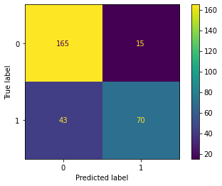
Lastly, I assess the model performance using the withheld validation data. I generate a confusion matrix and associated assessment metrics using sklearn. The model performed with an overall accuracy of 80% based on predicting to the withheld testing or validation data. The primary source of error was false negatives, or predicting that a passenger did not survive when he or she actually survived. Note the use here of the CunfusionMatrixDisplay() function from sklearn that produces a nice visualization of the error matrix.
predictions = ebm.predict(X_test)
cm = confusion_matrix(y_test.to_numpy(), predictions)
disp = ConfusionMatrixDisplay(cm)
disp.plot()
plt.show
<function matplotlib.pyplot.show(close=None, block=None)>
cr = classification_report(y_test.to_numpy(), predictions)
print(cr)
              precision    recall  f1-score   support

           0       0.79      0.92      0.85       180
           1       0.82      0.62      0.71       113

    accuracy                           0.80       293
   macro avg       0.81      0.77      0.78       293
weighted avg       0.80      0.80      0.80       293
Concluding Remarks
My goal here was to expand upon the last section, in which we investigate sklearn for implementing machine learning with Python. Here, we explored another package, interpretml, that provides functions for interpreting black box classifier and implementing more interpretable or explainable methods, such as EBMs. Here, we specifically explored the interpretable algorithms as opposed to the black box interpretation tools.
EBM is a nice tool for generating interpretable models with informative global and local output for explaining the model and local predictions. All components of the model are visualized with the provided graphics. If you are interested in implementing machine learning methods that are more interpretable but also provides strong predictive performance, please check out the EBM method.